What follows is my 2022 St Andrew's dissertation on applying a number of modern CPU optimization techniques to the simple 16-bit "Hack" platform described Noam Nisan and Shimon Schocken in their book "The Elements of Computing Systems" (Nand2Tetris). The book takes students on a journey of discovery, first implementing fundamental logic gates from NAND gates, then constructing a simple CPU from fundamental logic gates, and finally covering the full software stack from assembler to compiler to operating system. I highly recommend the book to anyone who wants to enhance their computer science knowledge from first principles.

PDF version here.

Abstract

Modern CPUs are extremely complicated devices making use of a variety of clever optimisation techniques. This project aims to provide an understanding of some of these optimisation techniques by implementing them on a simple computer architecture. The hardware platform Hack presented by Noam Nisan and Shimon Schocken in their 2005 textbook “The elements of computing systems” (also known as Nand2Tetris) was selected. After providing an overview of Hack and of 5 optimisations: memory caching, pipelining, pipeline forwarding, branch target prediction and branch outcome prediction, a simulator for the platform is developed. The simulator provides an elegant mechanism for developing CPU optimisations and is used to collect data so that the performance impact of each of the optimisations can be explored and compared. Data from 20,000 runs of the simulator is analysed and presented graphically. The contribution of this project is to compare and contrast some of the most important modern CPU optimisations.

Dedication

For Spike, who spent many an hour watching me work on this project and others. You will be missed.

Acknowledgements

Many thanks to Noam Nisan and Shimon Schocken for their excellent book, I found it hugely educational and interesting and it has changed my entire view of computers. Thanks to Shimon in particular for his email providing advice and encouragement regarding this project. I have tried to complete the book many times since I first acquired it over 10 years ago, eventually completing it after being inspired by Tom Spink’s Computer Architecture course at University of St Andrews. Many thanks to Tom for his outstanding course and all of his support, advice and expertise freely given during this project. As always, many thanks to my wonderful girlfriend and family for all their support and proof reading.

Introduction

Modern CPU designers rely on a range of clever optimisation techniques to improve the performance of their chips. This inclusion of so many optimisations on an already complex device makes understanding modern CPUs and CPU optimisations a challenge. This project aims to present a simple computer architecture and then implement some of the most important modern CPU optimisations on the simple platform. Once this has been done, the performance impact of each of the optimisations can be examined and compared.

The platform used in the project is called Hack and is a simple 16-bit Harvard architecture. Hack is simple enough to be built and understood by students in a matter of weeks, but complex enough to demonstrate the principles of modern computing systems. The optimisations that will be implemented on the platform are: memory caching, pipelining, pipeline forwarding and branch prediction.

As part of the project, a simulator for the platform will be developed. This simulator will provide an elegant mechanism for optimising various areas of the CPU. The simulator will provide a means to enable and disable each optimisation and set any related parameters. The simulator will also gather a variety of performance statistics regarding each run.

The rest of this report begins with a context survey discussing background information related to the project such as a detailed overview of the Hack platform, discussions on a number of optimisation techniques, benchmarking and cycles per instruction. This is followed by a detailed description of the simulator platform. Next, 15 benchmarks are defined to test the platform. After this, a more detailed look at each of the optimisations explored by this project is taken. This is followed by a deep dive into the results gathered by the project, explored through the use of data visualisation. An insightful evaluation of this data is provided, before some ideas for future work are presented and the report is concluded. This document includes 5 appendices. Appendix A provides links to the source code referred to throughout this report, appendices B and C provide a more detailed exploration of the hardware and software implementations of the Hack platform respectively, appendix D takes a brief look at some possible software optimisations and finally appendix E deals with the ethics of this project.

Context Survey

The Elements of Computing Systems

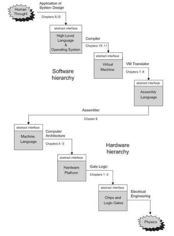
The Elements of Computing Systems [1] is a 2005 textbook written by Noam Nisan and Shimon Schocken. The authors assert that the complexity of modern computers and the segmented, specialised approach of a modern computer science education, deprive the student of a bigger picture understanding of how all of the hardware and software components of a computer system fit together. The authors aim to remedy this by providing students with an opportunity to build a computing system from first principles by gradually building a hardware platform and software hierarchy, as illustrated by Figure 2.

The platform constructed during the book is called Hack. Hack is a simple 16-bit Harvard architecture that can be built from elementary NAND gates and Data Flip-Flops. The instruction set is extremely simple with a focus on hardware simplicity. Programs are supplied to the computer in the form of replaceable ROM chips, similar to some cartridge-based games consoles. Despite this, the computer is powerful and building it is an extremely informative journey.

For the rest of this report, “The Elements of Computing Systems” will be referred to simply as “the book”.

Hack Architecture

Hack is a simple 16-bit Harvard architecture designed to be simple enough to be built and understood by students in a few weeks, but complex enough to demonstrate the inner workings of modern computer systems.

The platform is equipped with 3 physical registers and 1 "virtual" register. Memory is divided into program memory (ROM) and data memory (RAM). ROM can be read but not modified during runtime whilst the system has full access to RAM. Both ROM and RAM are addressed via two separate 15-bit address buses, meaning there are 32,678 possible locations in each unit. All 32,678 are available for ROM, giving a maximum program size of 32,678 instructions (although the simulator includes a mode enabling significantly more instructions). However, only 24,575 of these locations are available in RAM. Every memory location in both ROM and RAM, as well as each of the registers, are 16-bit two's compliment binary numbers.

The first of the 3 physical registers is a special register called the Program Counter (PC). The PC stores the address of the next instruction to be executed by the system. When execution of a new instruction begins, the instruction at ROM[PC] is fetched and the program counter is incremented by one. Programmers cannot directly manipulate the PC register, but it can be reset to 0 by asserting the CPUs reset pin, or indirectly manipulated through the use of jump commands.

The remaining physical registers are called A and D. The D register is a general-purpose data register, whilst the A register can be used as either a general-purpose data register, or as an address register. The M register is a "virtual" register that always refers to the memory location RAM[A]. Programmers can manipulate arbitrary memory locations by first setting the A register to the desired address and then reading or writing to the M register.

The RAM is divided up into two sections. The first section spans address 0 – 16,383, making it 16KB in size. This section is general purpose RAM and its exact usage is defined by the software implementation. The second section spans address 16,384 – 24,576 (8KB + 1 byte) and consists of two memory maps. The Hack platform is equipped with a 256 (height) by 512 (width) monochrome display. This screen is represented by the first memory map, which is 8KB in size and spans addresses 16,384 – 24,575. Each of these addresses represents a 16-pixel row, where a pixel can be illuminated by asserting the corresponding bit within the memory location. The pixel at row r (from the top) and column c (from the left) is represented by the c%16 bit of the word found at Screen[r*32+c/16]. The final address, 24,576, is a memory map representing the platform's keyboard. When a key is pressed, the corresponding key code is written to this memory location.

The instructions for the Hack platform are divided into two types: A-instructions and C-instructions. When written in assembly notation, A-instructions take the form:

@constant

Where constant is a positive integer. A-instructions are used to load constants directly into the A register. C-instructions take the form:

dest=comp;jump

As can be seen from the above, each C-instruction contains the fields dest, comp and jump. The dest and jump fields are optional, whilst the comp field is mandatory. This means that a C-instruction could also take the form:

dest=comp

Or:

comp;jump

Or even:

comp

Although this would not achieve anything and would be equivalent to a NOP (no operation).

The comp field instructs the ALU to compute a value which can be any of the mnemonics shown in Table 1, where !, | and & represent the logical NOT, OR and AND operators respectively.

Table 1 Assembly mnemonics for the comp field.

The dest field instructs the CPU where to store the output of the ALU. This field is optional and can be left blank, in which case the output will not be stored anywhere. If it is set, it can be any one or combination of the A, D and M registers.

The jump field instructs the CPU which instruction to execute next. This field is optional and can be left blank, in which case the CPU proceeds the next instruction as usual. If the field is set, it can hold one of 7 values shown in Table 2.

Table 2 Assembly jump mnemonic along with effect.

*Where out refers to the output of the ALU.

The software hierarchy of the Hack platform consists of five components: an assembler, a Virtual Machine (VM) translator, a high-level language compiler, an operating system and finally a program. The assembler, VM translator and compiler are all written in the Rust programming language, whilst the operating system and programs are written in the Jack programming language.

The assembler performs the job of translating the assembly language described above into binary machine code that the Hack platform can run directly. This is a trivial task, as each of the fields in a C-instruction have one-to-one mappings to binary, whilst A-instructions simply involve expressing the constant to be loaded as a 15-bit binary number. The task of the assembler is made slightly less trivial due to its support for symbols. The Hack assembly language supports two types of symbols: labels and variables. Labels are used to refer to another part of the program and are translated to program memory (ROM) addresses. The assembler relieves the programmer of the burden of manually assigning and keeping track of which variables refer to which memory locations by supporting variable symbols.

Whilst it is possible to compile directly from a high-level language (such as Jack) to assembly, today it is more popular to first translate the high-level language into an intermediate language, then later translate the intermediate language to assembly. This approach enables abstraction, reducing the amount of work the compiler must do and also improves portability. The Hack platform specifies a stack-based Virtual Machine (VM) that runs an intermediate language referred to as VM language/code. The stack-based nature of the VM implementation provides an intuitive mechanism for function calling and elegantly handles most of the memory management needs of the system. Some VM implementations, such as the Java VM, act as an interpreter/runtime for the VM code. This differs to the approach taken by this project as the VM translator program has the job of translating VM code into assembly code that exhibits the same behaviour and the VM code simply acts as an intermediate representation.

The compiler used in this project translates programs written in Jack into programs that can run on the VM implementation described above. The Jack programming language is a simplistic, weakly-typed, object-oriented, C-like language. Both the operating system and the programs that run on the Hack platform are typically written in Jack, although there’s no reason a compiler for another programming language couldn’t be implemented for the Hack platform. All of the benchmarks used as part of this project have been written in Jack.

Modern Operating Systems (OS) are typically extremely complicated programs that must offer a wide variety of services to programs running on top of them, whilst also managing the system’s resources and enabling multiple programs (and possibly users) to run simultaneously and without interfering with each other. Luckily the OS utilised in this project does not need to be as complex, due in no small part to the fact that Hack platform is single-user and single-tasking. Our OS does not even need to be capable of loading programs as all programs are supplied in the form of replaceable ROM cartridges. In fact, the OS utilised by this project is more of a standard library for the Jack programming language then it is an OS. This is the only part of the project that has not been implemented (yet!) by the author. The OS used in this project is called Jack OS and is supplied with the book.

For more information on the hardware or software platform, please see Appendix B: Hardware Implementation or see Appendix C: Software Implementation respectively.

Optimisations

Hardware designers and CPU architects are in a constant race to build the fastest possible processors. Whilst performance improvements can come from increasing clock speeds and reducing the size of the underlying transistors, most performance improvements come from efficient design and clever optimisations. Hardware manufacturers must compete to build the highest performance chips at the lowest possible price and are therefore constantly looking for new ways to optimise their designs. General purpose CPUs are exposed to a significant and varied volume of code, some of which is badly written, which makes optimisations at a hardware level even more important. This is partly because the hardware designers do not know ahead of time exactly what the CPU will be used for and must be reasonably confident that the CPU will be able to handle its workload efficiently. Even when the code being executed is well written, there is only so much that can be done through software optimisations. Table 3 below summaries a number of optimisation techniques employed in modern CPUs.

Table 3 CPU optimisations summary.

Benchmarks

Benchmarks are used to enable comparison between CPUs by scoring their performance on a standardized series of tasks [20]. Benchmarks are essential to evaluating the performance improvement derived by implementing an optimisation. Benchmarks can be broadly divided into two categories: synthetic and real-world. Synthetic benchmarks require the CPU to complete a series of tasks that simulate a high-stress workload. Examples of synthetic benchmarks include:

• PassMark: runs heavy mathematical tasks that simulate workloads such as compression, encryption and physics simulations
• 3DMark: measures the system ability to handle 3D graphics workloads
• PCMark: scores the system on how well it can deal with business workflows

Real-world benchmarks are carried out by giving real programs a heavy workload and then measuring the amount of time taken to complete the task. Popular programs to run real-world benchmarks on include:

• 7-Zip: measure the CPU’s compression and decompression performance
• Blender: measure the CPU’s 3D rendering speeds
• Handbrake: measure the CPU’s video encoding speed

Synthetic benchmarks typically nest a code snippet within a loop. Timing libraries are used to measure the amount of time elapsed per iteration of the loop. The loop is run many times and elapsed time averaged in order to control for outliers [19].

In addition to dividing benchmarks into synthetic and real-world categories, benchmarks can also be divided into micro and macro benchmarks. All of the benchmarking techniques discussed so far have been macro benchmarks. Macro benchmarks aim to test the performance of the entire CPU. In contrast, micro benchmarks aim to test only a single component of the CPU. This can be useful when evaluating the effect of parameters or strategies within a single component of the CPU.

SPEC CPU 2017

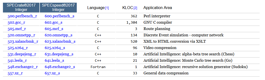
The Standard Performance Evaluation Corporation (SPEC) produce a number of benchmarking tools targeting a number of different computing domains [21]. Their CPU package includes 43 benchmarks based on real-world applications (such as the GCC compiler) and organised into 4 suites. The suites are SPECspeed 2017 Integer, SPECspeed 2017 Floating Point, SPECrate 2017 Integer and SPECrate 2017 Floating Point. The SPECspeed suites compare the time taken for a computer to complete single tasks, whilst the SPECrate suites measure throughput per unit of time. The Hack platform is not equipped with floating point units and any support for fractional values would have to be implemented in software, therefore only the integer benchmarks are of interest for this project. The programs that make up the SPEC integer suites are shown in Figure 3. More information can be found on the SPEC website [21] and the source code for each benchmark can be obtained by purchasing a SPEC licence. Note that KLOC refers to the number of lines of source code divided by 1000.

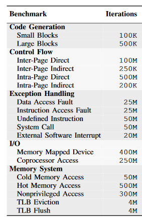
SimBench

SimBench is a benchmark suite specifically designed to test the performance of CPU simulators [17]. SimBench was proposed in 2017 by Wagstaff et al., after noting that more traditional benchmarking suites such as SPEC are not able to identify specific bottlenecks in a computer architecture simulator. 18 benchmarks are included in the suite and these benchmarks are organised into five categories: Code generation, Control Flow, Exception Handling, I/O and Memory System. Figure 4 shows the benchmarks making up SimBench. Wagstaff et al. includes a detailed description of each of the benchmarks and the source code is available fromhttps://github.com/gensim-project/simbench.

Cycles per Instruction

Every instruction within a CPU’s instruction set will require a certain number of cycles to complete. Different instructions may take a different number of cycles to complete. For example, an add instruction may take 2 cycles whilst a divide instruction could take 20 cycles to complete. Memory accesses typically take the most cycles to complete. The number of cycles it takes to complete a given instruction is called Cycles per Instruction (CPI). Average CPI (across all instructions) is often used as a performance metric as it describes the average number of cycles required to complete an instruction. Since a cycle is effectively the CPUs base time unit, average CPI gives a good indication of what latency can be expected for an instruction.

Table 4 shows the CPI for a number of common operations for the Intel 8086, Intel 10^th Generation Core and AMD Ryzen 3700. The timings for the Intel 8086 are taken from Liu et al. [22] whilst the timings for Intel 10^th Generation Core and AMD Ryzen 3700 are taken from A. Fog [23]. The operations most relevant to the Hack platform have been selected. For purposes of simplicity the following assumptions have been made:

• Operations can only be performed on register operands.
• Memory can only be accessed by explicitly loading a value into a register from memory and explicitly saving a value from a register into memory (using MOV).
• If an instruction has multiple variants for different bit lengths, the native bit length will be used. I.e., the DEC operation on the intel 8086 has an 8-bit and 16-bit variant, as the 8086 is a 16-bit processor, the 16-bit variant will be used.
• Where indirect and direct addressing modes are available, direct addressing has been used.

Some of the values in the table are ranges, this is because the number of cycles required to complete an instruction may be dependent on the architectural state of the system or the operands supplied to the instruction. Factors may include whether a prediction was correct, state of the memory cache or size of the operands.

Table 4 Comparison of CPI for a number of instructions across 3 different CPUs.

Simulator

The simulator is the centrepiece of this project as it enables a variety of optimisations to be experimented with without requiring the physical construction of a new computing system. The simulator developed in this project was programmed in the Rust programming language and development involved iterating through 3 generations.

First-Generation Simulator

The first attempt at a simulator operated on unassembled Hack assembly programs instead of directly on binaries. This meant that it had to also carry out some of the functions of an assembler, such as maintaining a symbol table. This also meant that the simulator was carrying out a large number of string comparisons.

The first-generation simulator emulated exactly 1 instruction per cycle. The screen and keyboard peripherals were simulated using the Piston [24] rust library and this was done in the same thread as the rest of the simulator. This resulted in a trade-off between screen/keyboard updates per second and the speed of the rest of the simulator. At 15 updates per second, the simulator was able to achieve a speed of 10,000 instructions per second.

Second-Generation Simulator

The second-generation simulator looked to address a number of shortcomings with the first-generation simulator. Firstly, it operated directly on assembled binaries, which eliminated the requirement for assembler functions such as the symbol table and also removed the need for any string comparisons, significantly reducing overhead. The use of Piston for screen and keyboard simulation was replaced by the Rust bindings for the SDL2 library [25]. More significantly, the screen and keyboard peripheral simulation was moved into a separate thread, meaning that the updates per second for these devices was independent of the instruction rate for the rest of the simulation. These improvements enabled the simulator to achieve a significantly faster simulated clock speed of 5 million cycles per second at 144 peripheral updates per second.

During the development of the first-generation simulator, it was noticed that many of the programs provided by the book and once built using the toolchain (described in Appendix C: Software Implementation) were too large to fit into the 32K ROM chip. In order to combat this problem, a 32-bit mode was added to the second-generation simulator. Whilst attempts will be made later in the project to reduce the size of compiled binaries (Appendix D: Software optimisations), it would be a fairly simple undertaking to convert the Hack platform to 32-bits, for the most part simply involving replacing 16-bit registers with 32-bit registers and increasing the bus widths to 32-bits. A 32-bit Hack platform also has the benefit of having more unused bits in its C-instruction which could enable the addition of new instructions later in the project.

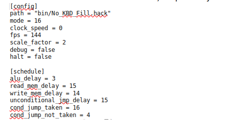
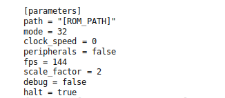
Another important improvement in the second-generation simulator was the addition of simulated cycle delays for various operations such as imposing a 3-cycle delay for the ALU to compute an output. These delays, along with a number of other parameters, could be configured in a file such as the one shown in Figure 5. The parameters in the config section of file enable the user to specify the path to the program ROM they wish to run, specify 16- or 32-bit mode, specify a target clock speed (0 for unlimited), specify the number of frames/updates per second, specify a scale factor for the screen, turn debug mode on or off (which results in debug messages being output to the display) and turn halt detection on or off (which detects once the OS function halt is called and terminates the simulation) respectively.

Third-Generation Simulator

The third-generation simulator is very similar to the second-generation simulator in terms of performance and peripheral simulation. The key improvement for the third-generation simulator is splitting the simulated CPU up into 8 modules:

• Control Unit: Responsible for scheduling instructions and conducting the remaining modules
• A-Instruction Unit: Responsible for loading the constant from an A-Instruction
• Memory Unit: Responsible for reads and writes to main memory
• Operand Unit: Responsible for retrieving the x and y operands for the comp field of a C-instruction
• Arithmetic Logic Unit: Responsible for executing the comp field of a C-instruction
• Jump Unit: Responsible for executing the jump field of a C-instruction
• Write Back Unit: Responsible for saving values into the A, D and M registers and carrying out the dest field of a C-instruction.
• Decode Unit: Responsible for decoding instructions prior to executing them.

Each module is represented by a trait (similar to an interface in other programming languages) which must be replaced by a concrete implementation at runtime. This enables new optimisations to be implemented simply by writing a trait implementation for the relevant module. For example, when implementing a memory cache, only the Memory Unit would need to be rewritten, rather than producing a completely new simulator as previous generations of the simulator would require.

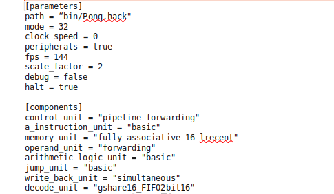
The third-generation simulator also takes a configuration file to specify the various parameters of simulation. The first section of the configuration file is similar to the second-generation configuration file, only the section has been renamed parameters and there is an additional parameter, peripherals, which can be used to turn the peripherals on or off. Instead of specifying a schedule of delays as in the second-generation simulator, the third-generation simulator allows users to specify which implementation for each of the 8 modules to use. An example of a third-generation configuration file is shown in Figure 6.

Benchmarks

The performance of the base system and various configurations of optimisations will be evaluated across a suite of benchmarks. The benchmark suite includes two “real-word” macro benchmarks taken from the book and described in detail below. In addition to this, 13 micro “synthetic” benchmarks were developed as part of this project and are described in Table 5.

Seven

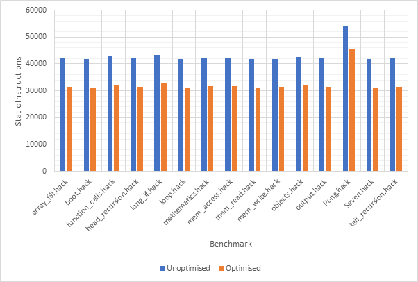
Seven is one of the test programs supplied by the book. It is written in Jack and evaluates a simple expression and then displays the answer on the screen. The program makes use of the full software stack including some of the operating system routines. The assembled binary contains 41809 instructions. Along with testing the operating system boot procedure and a few of the standard library functions, the Seven program tests some of the basic features of the Jack programming language.

Pong

During initial testing of the simulators and to gain an idea of the improvement achieved by implementing various optimisations, the Pong program supplied by the book was used. Although this is an interactive game, the game will always end after the same number of cycles as long the user does not supply any input. Under these conditions, the program is deterministic. The Pong program is the most advanced program supplied by the book and uses most of the features of the Jack programming language and OS. The assembled binary for the Pong program is 54065 static instructions. Pong provides the closest to a real-world application that a user of a simple computer like the Hack platform would be likely to encounter.

Table 5 13 micro synthetic benchmarks

*Static

Staged Instructions (Base Model)

This section attempts to define a realistic schedule for how many cycles each instruction should take to complete based on the timings of the Intel 8086 shown in Table 4. This is done by splitting each single instruction into 4 stages and defining how many cycles each of these stages should take to complete in various circumstances. Taken together, this forms the base model which the optimisations in the remainder of this project attempt to improve upon.

The four stages are Instruction Fetch, Instruction Decode, Execute and Write Back. The execute stage consists of 1 sub-stage in the case of an A-instruction, or 3 sub-stages in the case of a C-instruction (Operand Fetch, Computation and Jump). These stages are loosely based on the classic RISC 5-stage pipeline [26, 27], however cannot be considered a true “pipeline” yet, as only one instruction can occupy the pipeline at any one time. This one instruction can only be in one of the 4 stages at any given time and the remaining stages will be empty. When an instruction is executed, the control unit orchestrates the execution of each of the stages sequentially by instructing the various modules making up the CPU. Figure 8 summaries the various stages, note that A-instructions follow the top route along the Execute stage, whilst C-instructions follow the bottom route. Each stage is described in more detail in below. The system described in this section can be simulated by setting the control_unit parameter to “staged”.

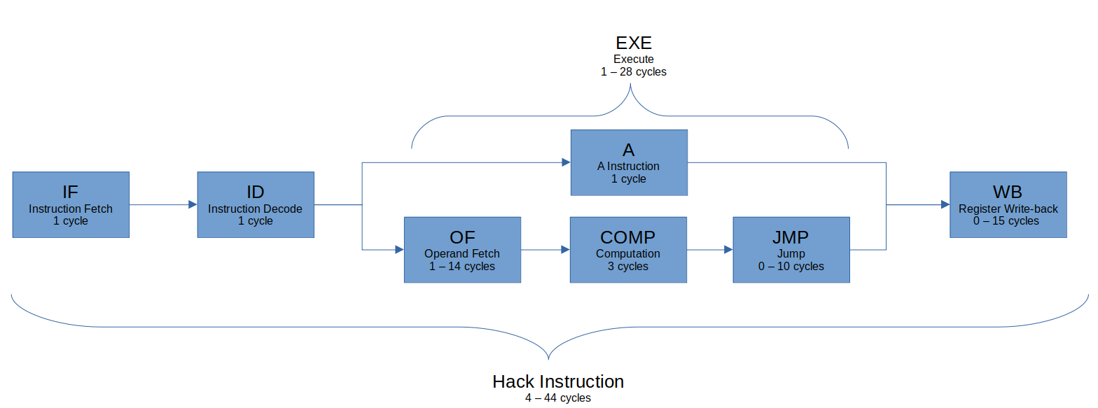
IF – Instruction Fetch

• Completes in 1 cycle
• Retrieves the next instruction from ROM
• Increments the PC by 1

ID – Instruction Decode

• Completes in 1 cycle
• Determine if A or C instruction

EXE – Execute

• Completes in 1 – 28 cycles
• A-instruction: 1 stage (A) completes in 1 cycle
• C-instruction: 3 stages (OF, COMP, JMP) completes in 4 – 28 cycles

A – A Instruction

• Completes in 1 cycle
• Loads constant from instruction

OF – Operand Fetch

• Completes in 1 – 14 cycles
• Available operands: A, D, M
• If comp field refers to M, load value from RAM[A] (14 cycles)
• If comp field refers to A and/or D, load value from A and/or D (1 cycle)

COMP – Compute

• Completes in 3 cycles
• ALU computes output based on operands and control inputs (instruction)

JMP – JUMP

• Completes in 0 – 10 cycles
• Optionally transfers control to another part of the program
• If jump field unset, completes in 0 cycles
• If jump field set:
  • Unconditional Jump: Set PC to value in A register (4 cycles)
  • Conditional Jump: Determine if jump should be taken based on ALU flags (6 cycles):
    • Taken: Set PC to value in A register (4 cycles)
    • Not taken: No further action (0 cycles)

WB – Write Back

• Completes in 0 – 15 cycles
• Optionally write ALU output to (any combination of) A, D, M
• If A-instruction, write to A
• If C-instruction, proceed based on dest field
• If dest field unset, completes in 0 cycles
• If dest field contains A and/or D, completes in 1 cycle
• If dest field contains M, writes to RAM[A] and completes in 15 cycles

Pipeline

As the reference to the RISC 5-stage pipeline may have suggested, the staged instruction approach laid out in the previous section is positioned perfectly for a pipelined approach. Rather than waiting for an instruction to pass through all 4 stages before repeating the process for the next instruction, with only slight modifications, the system is able to process 4 instructions simultaneously, with one in each stage. This will be the first hardware level optimisation proposed by this project and will form the foundation for many of the other optimisations explored later in the project.

Under the pipeline approach, when instruction_i is in the IF stage, instruction_i-1 is in the ID stage, instruction_i-2 is in the EXE stage and instruction_i-3 is in the WB stage. For a simplified pipeline, where each stage takes exactly 1 cycle, this is shown in Figure 9.

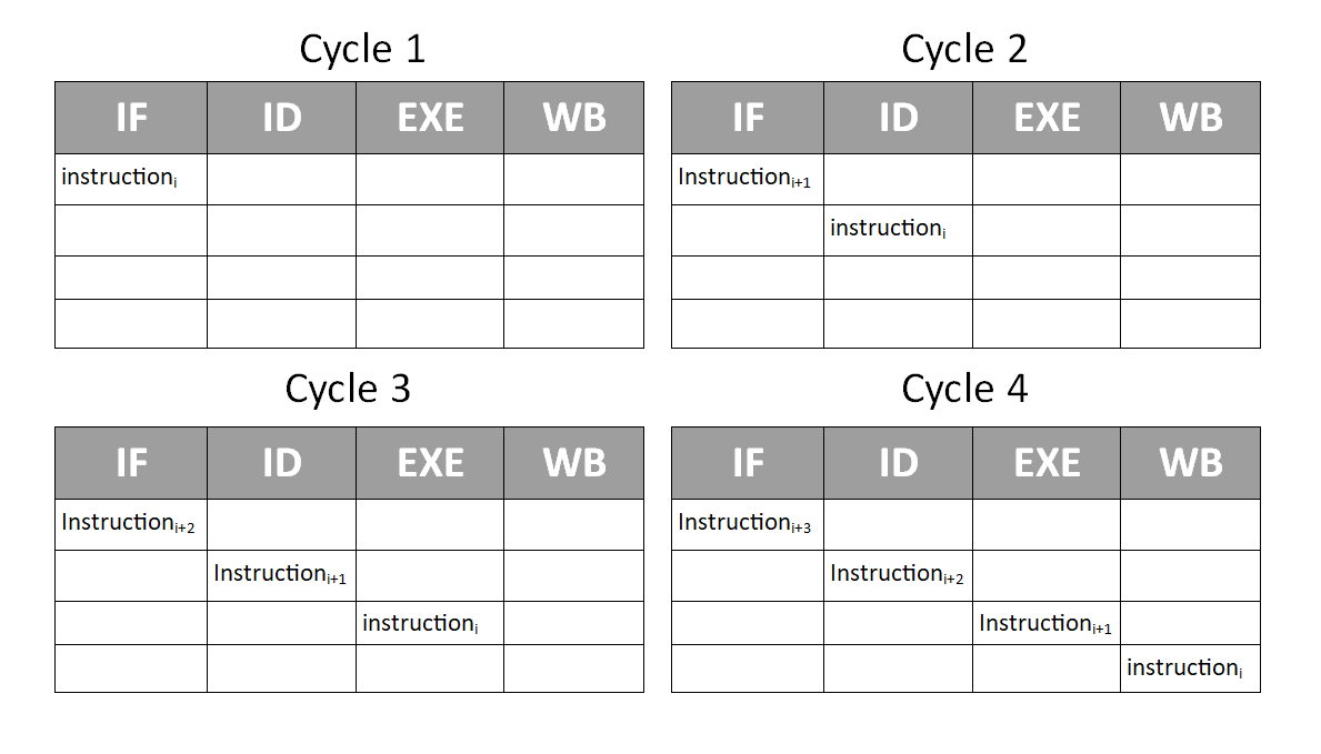
All of the changes required to implement this pipelined approach can be implemented in the control unit module. The pipelined control unit must orchestrate the various processing unit modules making up the stages such that all four are (nearly) always busy. As well as tracking the contents of the each of the stages control unit must take action to avoid two major hazards.

The first hazard occurs when a jump is taken. When an instruction causes a jump to happen, the control unit is not aware of this until after the JMP sub-stage of the EXE stage, by which point it will have already decoded and fetched the next two instructions directly following the instruction causing the jump. Since a jump instruction transfers control to another part of the program, these two instructions should not be executed. In this case, a pipeline flush or simply a flush occurs. During a flush, the contents of the IF and ID stages are discarded and no further instruction is fetched until the contents of the EXE and WB stage have completed. A flush should be triggered whenever an unconditional or conditional jump that is taken occurs.

The second hazard occurs when an instruction reads from a register that an instruction in the EXE or WB stage is simultaneously writing to. In this case, the decode stage must stall the pipeline until the relevant instruction has completed the WB stage. When the pipeline is stalled, no further instructions can enter the IF, ID or EXE stages, but instructions already in the EXE stage may continue, whilst instructions are free to enter and execute the WB stage as usual. The decode stage stalls the pipeline if it is decoding a C-instruction and the following conditions are met:

• If any instruction in pipeline is an A-instruction or a C-instruction writing to the A register AND:
  • Current instruction operates on A register OR
  • Current instruction operates on M register OR
  • Current instruction writes to M register
• If any instruction in pipeline is a C-instruction writing to the D register AND:
  • Current instruction reads from D register
• If any instruction in the pipeline is a C-instruction writing to the M register AND:
  • Current instruction reads from M register

The system described in this section can be simulated by setting the control_unit parameter to “pipeline”.

Pipeline Forwarding

Pipeline forwarding is an optimisation technique where earlier stages are able to take advantage of information produced by later stages in order to gain a cycle advantage. Two pipeline forwarding techniques are utilised in this project, which are discussed below. In order to take advantage of these techniques, a new forwarding-enabled control unit is required. To enable the forwarding-enabled control unit, set the control_unit parameter to “pipeline_forwarding”. Note that the pipeline forwarding control unit is also capable of branch predictions.

Simultaneous write back

In the original pipeline model, the write back stage occurs after the jump sub-stage of the execute stage has completed. The computation sub-stage of the execute stage determines the output, out of the ALU. The jump stage sets the program counter based on out and the write back stage writes out to any one (or none) of the 3 registers. Hopefully the reader can see that these two steps are mutually independent – both require out to be ready, but do not modify it. For instructions that contain possible branches, the simultaneous write back optimisation takes advantage of these facts and performs both the jump sub-stage and the write back stage at the same time. Since both stages have to potential to take a significant number of cycles, performing them simultaneously has the potential to greatly increase instruction throughput. The write_back_unit parameter should be set to “simultaneous” to employ this technique.

Operand Forwarding

In the original pipeline model, if the decode stage encounters any instructions which rely on registers being modified by instructions in the execute or writeback stage, the pipeline is stalled until the later instructions have completed. This is because the operand fetch sub-stage of the execute stage cannot begin until all the registers it will access have been updated. The operand forwarding technique attempts to alleviate this problem by allowing the operand unit to retrieve the updated values for dependent registers directly from the write back unit, without waiting for it to finish writing this data back to the relevant register. This has the potential to reduce the amount of time the CPU spends stalled. Instructions are no longer stalled when dependent on an instruction in the write back stage and instructions dependent on an instruction in the execute stage are only stalled until that instruction enters the write back stage. However, this creates another problem – it is possible for memory reads (by the operand unit) to occur at the same time as memory writes (by the write back unit). This is alleviated by adding an additional memory unit, using one as a dedicated writer and the other as a dedicated reader. This solution has the side effect of creating two independent memory caches (if memory caching is enabled). The operand_unit parameter should be set to “forwarding” to employ this technique.

Memory Caches

Based on the figures presented in Table 4, main memory is very slow, taking 15 cycles to write a value and 14 cycles to read a value. Therefore, the CPU would significantly benefit from having access to a bank of faster memory. All the memory caches simulated in this project are able to provide 1 cycle read/write access to any memory addresses that are “cached”.

Static Memory Cache

The static memory cache is the most basic memory cache explored in this project. The static memory cache caches the first x memory locations of the main memory, where x is the size of the cache. As the VM implementation frequently accesses data stored in the first 16 locations (e.g. location 0 is the Stack Pointer), substantial performance improvements are on offer. The static memory cache can be enabled by setting the memory_unit parameter to “static_x” where x is the desired size of the static cache.

Direct Mapped Cache

Direct mapped caches are the simplest class of caches that are able to cache any memory location within the main memory. Each memory location in the main memory is mapped to a single cache line in the memory cache. The exact cache line index is found by looking at the last x bits of the memory address, where x is log₂ of the cache size. This index is determined by applying a bitwise AND mask to the memory address. When an address is accessed, if the address is currently cached, it can be accessed in a single cycle. If not, the access takes the standard number of cycles, but the address is brought into the cache ready for future accesses. If the relevant cache line is already occupied (capacity miss), the original occupant is evicted and replaced with the new address. The direct mapped cache can be enabled by setting the memory_unit parameter to “direct_mapped_x” where x is the desired size of the direct mapped cache.

N-Way Set Associative Cache

In a set associative cache, the cache is organised into sets, where each set contains a number of cache lines. The set associative cache has two parameters, size and ways. The ways parameters specifies the number of cache lines in each set. Therefore, the number of sets is determined by dividing size by ways. For example, a 2-way 16 line set associative cache would have 8 sets. Each memory location in main memory is mapped to a single set, however could occupy any of the lines within that set. The set index is found by looking at the last x bits of the memory address, where x is log₂ of the number of sets, this is also determined using a bitwise AND mask. This organisation increases the complexity of the cache, but reduces conflicts and therefore capacity misses. Much like the direct mapped cache, when an address is accessed, if the address is currently cached, it can be accessed in a single cycle. If not, the access takes the standard number of cycles, but the address is brought into the cache ready for future accesses. If the relevant set has an unoccupied cache line, the address is brought into that empty line. If, however, the set is already fully occupied, one of the existing occupants is evicted and replaced by the new address. The cache line to be evicted is determined by the cache eviction policy. Note that a direct mapped cache is a 1-way set associative cache. The direct mapped cache can be enabled by setting the memory_unit parameter to “n_way_set_associative_x_y” where x is the desired number of ways and y is the desired size of the n-way set associative cache.

Fully Associative Cache

In a fully associative cache, any memory location can be cached in any cache line. This scheme offers the most flexibility and therefore the least capacity misses, however is the most complex cache and hence the most difficult/expensive to implement in hardware. In the real world, this additional complexity usually comes at a cost – longer lookup time when compared with other caches. This additional lookup time has not been considered in these simulations. As with the previous two caches, when an address is accessed, if the address is currently cached, it can be accessed in a single cycle. If not, the access takes the standard number of cycles, but the address is brought into the cache ready for future accesses. If there is an unoccupied cache line anywhere within the cache, the address is brought into that cache line. If not, one of the cache lines is evicted and the new address is brought into that cache line. The cache line to be evicted is determined by the eviction policy. Note that a fully associative cache is a special case of the n-way set associative cache, where n is equal to the size of the cache. The fully associative cache can be enabled by setting the memory_unit parameter to “fully_associative_x” where x is the desired size of the fully associative cache.

Eviction Policies

Eviction policies are used to determine which cache line should be evicted to make way for a newly accessed memory location. These policies are employed by the N-way set associative cache to determine which cache line within a set should be evicted, whilst they are employed by the fully associative cache to decide which cache line within the entire cache should be evicted.

FIFO

When using the First In, First Out (FIFO) eviction policy, cache lines are organised into a queue in the order they were brought into the cache. When a new address is cached, it is placed at the back of the queue. When it is time to evict a cache line, the cache line that was occupied least recently and is therefore at the front of the queue, is evicted.

LIFO

The Last In, First Out (LIFO) eviction policy is similar to the FIFO eviction policy in that cache lines are still organised into a queue in the order they were brought into the cache. However, when it is time to evict a cache line, the cache line that was occupied most recently and is therefore at the back of the queue is select for eviction.

Least Recent

The least recent eviction policy also organises cache lines into a queue, however unlike the previous two policies, the queue is ordered by when the cache line was last accessed rather than when it was brought into the cache. This means that when accessing an address that has already been cached, the cache line is moved to the back of the queue. When it is time to evict a cache line, the cache line at the front of the queue is selected. This means the cache line that was accessed least recently is evicted.

Most Recent

The most recent eviction policy is similar to the least recent eviction policy; however, it evicts the most recently accessed cache line instead of the least. The cache lines are kept in a queue following the same rules as the least recent policy, but evictions are made from the front of the queue instead of the back.

Branch Prediction

Under the standard pipeline model, the pipeline must be flushed every time a branch is taken. This is because the fetch and decode stages will already contain instructions i+1 and i+2 when it should contain instructions t and t+1, where i is the (program counter) address of the instruction containing the jump and t is the target address of the branch. This situation arises because the fetch and decode stages are unaware that there will be a jump in instruction i until the execute stage has concluded for that instruction, by which time they will already have loaded the subsequent instructions i+1 and i+2.

Branch prediction is an optimisation technique that attempts to alleviate this problem. During the decode stage, the decode unit determines if an instruction contains a branch. If it does contain a branch, the decode unit makes a prediction about the outcome of the branch (taken or not taken). Unconditional jumps are always predicted to be taken.

If the jump is predicted not taken, then no further action is taken and the program proceeds to the next instruction as normal.

If the jump is predicted to be taken, then the decode unit also makes a prediction about the target of the jump. The program counter is then updated to the predicted target of the jump and a “half-flush” is triggered. During a “half-flush” only the fetch unit is cleared. During the next cycle, the fetch unit will fetch the next instruction from the predicted target address.

Once the execute stage concludes, the actual branch outcome and branch target are compared to their predictions. If they are equal, then no further action is needed and a number of cycles are saved. If the predictions were wrong, then a pipeline flush is triggered so that the correct instructions can be retrieved. Therefore, the flush is avoided as long as both the outcome and target prediction are correct.

Note that most modern architectures support both direct and indirect branches. In a direct branch, the branch target is contained within the branch instruction. During an indirect branch, the branch target is contained elsewhere, typically within a register. This means that branch target prediction is only needed for indirect branches. However, the Hack architecture only supports indirect branching – the branch target is always the value of the A register at the time the jump is taken. As a result, for the Hack architecture, branch outcome prediction is only useful when employed in combination with branch target prediction.

Branch prediction requires changes to both the control and decode units. The prediction-enabled pipeline can be enabled by setting the control_unit parameter to “prediction_pipeline” in the simulator configuration. There are a number of different outcome and target prediction strategies, which are discussed below. These can be enabled by setting the decode_unit parameter to the relevant strategy. However, as discussed previously, it is not useful to have an outcome predictor without a target predictor, so both an outcome and target strategy should be specified. This can be done by including both strategies within the decode_unit parameter, separated by an underscore, e.g., “gshare16_fifo2bit16”.

Branch Outcome Prediction

A branch outcome predictor produces a prediction of either taken or not taken for a given instruction address (prediction). After the branch is fully resolved, the predictor is told the actual outcome of the branch so that it can make any relevant updates (confirmation).

Never Taken

This is the simplest prediction strategy and in fact is the behaviour already exhibited by the pipeline. Branches are always assumed to be not taken and the instruction after the branch instruction is loaded. The only benefit to this strategy over not using the prediction-enabled pipeline is that target predictions will be made and acted upon in the case that the branch is unconditional if a target predictor has been enabled. The never taken strategy ignores any confirmations it receives and is therefore a static strategy. The decode_unit parameter should be set to “nevertaken” to employ this strategy.

Always Taken

The always taken strategy predicts taken in all circumstances. Like the never taken strategy, it ignores all confirmations and is therefore a static strategy. This strategy should be correct approximately 50% of the time, however this will depend on the program being executed. If the compiler is aware that the always taken strategy is in use, code can be reorganised to take advantage of the fact that all branches will be assumed to be taken. The decode_unit parameter should be set to “alwaystaken” to employ this strategy.

Global 1-bit predictor

The global 1-bit predictor is the first dynamic branch prediction strategy explored by this project. This predictor simply predicts the same outcome as the last branch that was taken (regardless of instruction address). This is done by storing the outcome of the last branch and returning when a prediction is requested. This outcome is updated when receiving a confirmation. The decode_unit parameter should be set to “global1bit” to employ this strategy.

Global 2-bit predictor

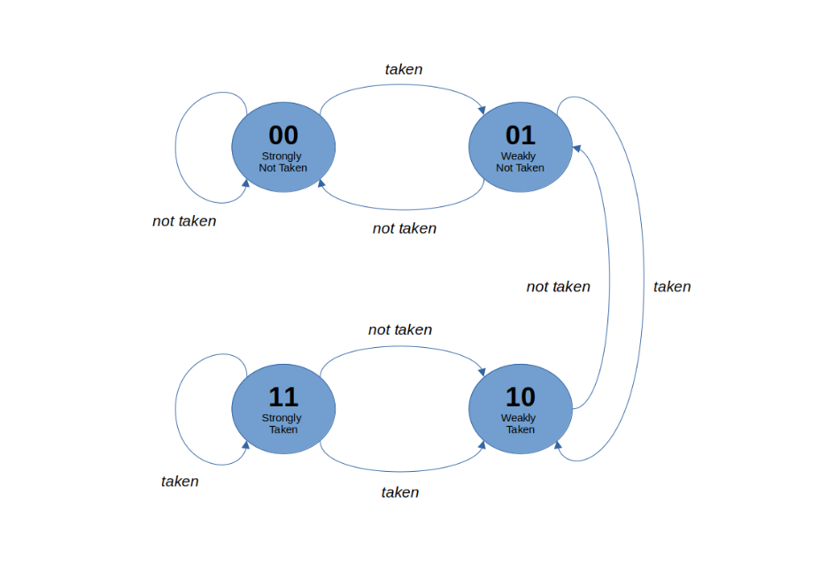
The global 2-bit predictor is a dynamic strategy similar to the global 1-bit predictor. This predictor utilises a 2-bit saturating counter. This 2-bit counter capable of storing the values 0-4 (inclusive). If the counter is 0 or 1, the predictor will predict not taken, whilst if the counter is 2 or 3, the prediction is taken. When a confirmation is received, the counter is incremented if the branch was in fact taken and decremented if it was not. This is illustrated in Figure 10. When compared to the 1-bit prediction strategy, this has the benefit of making the prediction more stable by requiring two mispredictions in a row in order to change the predicted outcome. The decode_unit parameter should be set to “global2bit” to employ this strategy.

Local 1-bit predictor

The local 1-bit predictor is a dynamic strategy that holds a prediction table of a size specified by the size parameter. Each (program memory) address is mapped to one of the cells in the table. The specific table index is found by looking at the last x bits of the address where x is equal to log₂ of the table size and is determined using a bitwise AND mask. Each cell contains a boolean prediction, equal to the outcome of the last branch instruction that had an address mapping to the same cell. This outcome is updated when a confirmation is received. The decode_unit parameter should be set to “local1bit[size]” to employ this strategy, where [size] should be replaced by the desired table size.

Local 2-bit predictor

The local 2-bit predictor is a dynamic strategy similar to the local 1-bit predictor strategy in that is also holds a prediction table and each address is mapped to one of the cells in the table. However, instead of storing a boolean outcome in the table, a 2-bit saturating counter is stored. This counter is updated in the same way as the 2-bit global strategy. The decode_unit parameter should be set to “local2bit[size]” to employ this strategy, where [size] should be replaced by the desired table size.

Gshare

Gshare or Global Sharing, is a dynamic strategy that attempts to combine the benefits of the global and local predictors, by employing a hybrid approach enabling it to leveraging both global and local information. Gshare also holds a prediction table of a size specified by the size parameter, when each cell contains a 2-bit saturating counter. In addition to this, the gshare predictor maintains a global history (shift) register (GHR). This register stores the outcomes of every branch in the form of a binary number where each digit represents a taken (1) or not taken (0) outcome. When the predictor receives a confirmation, it updates the GHR by shifting it one place to the right and then setting the last bit to true if the outcome was taken and leaves it as false if not. The relevant 2-bit counter in the prediction table is also updated. The index to the prediction table is found by XORing the last x bits of the (program memory) address and the last x bits of the GHR, where x is log₂ of the size of the prediction table. The decode_unit parameter should be set to “gshare[size]” to employ this strategy, where [size] should be replaced by the desired table size.

Branch Target Prediction

A branch outcome predictor produces a target address prediction for a given instruction address (prediction). After the branch is fully resolved, the predictor is told the actual target address of the branch so that it can make any relevant updates (confirmation).

1-bit target predictor

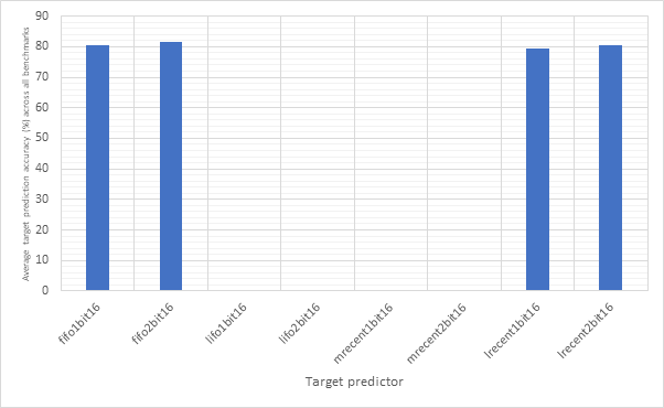
The 1-bit target predictor acts similarly to a memory cache. It maintains a target buffer of a size specified by the size parameter. Each entry in the buffer contains an instruction address and the target address of that instruction last time it was executed. When a confirmation is received, this target address is updated. If a prediction is requested for an address that is not already in the cache, a prediction of target address 0 is produced and the address is added to the buffer so that it is ready for next time. In this way, the target buffer stores the last size branch instruction and their targets. If a new address is added when the buffer is full, one of the existing entries is evicted according to the selected eviction policy. The policies available are the same as the ones used by the set associative and fully associative memory caches. The decode_unit parameter should be set to “[eviction_policy]1bit[size]” to employ this strategy, where [eviction_policy] should be replaced by the desired eviction policy (fifo, lifo, mostrecent or leastrecent) and [size] should be replaced by the desired table size.

2-bit target predictor

The 2-bit target predictor is similar to the 1-bit target predictor: it also maintains a target buffer of a size specified by the size parameter, uses the same eviction strategies to make room once the buffer is full and when a prediction is requested, the addresses is looked up in the cache and the respective target address is produced, or 0 if the address does not appear in the target buffer. However, in addition to storing the instruction address and target address in the buffer, a 2-bit counter is also stored. When a confirmation is received, the counter is incremented by 1 if the predicted target was correct and decremented by 1 if it was wrong. The stored target is only updated once the counter reaches 0. When a target is updated, or a new entry added to the target buffer, the counter is (re)initialised to 1. The decode_unit parameter should be set to “[eviction_policy]2bit[size]” to employ this strategy, where [eviction_policy] should be replaced by the desired eviction policy and [size] should be replaced by the desired table size.

Results

Methodology

This section aims to use graphs and explanatory text to showcase, explore and compare the effects of the optimisations discussed in this project. This has been done by statistically analysing performance data generated during simulated runs of various different configurations. Each of the configurations have a different combination of optimisations enabled.

Two python scripts were developed for the purposes of gathering data. The source code for both of these scripts can be found in Appendix A: Links. The first script, generate_configs.py, is used to generate batches of simulator configurations where each configuration is one permutation of the possible CPU components paired with one of the benchmark programs. Each possible permutation has one simulator configuration for each of the 15 benchmarks. The components included in these permutations are specified as a parameter. The second script benchmarker.py is used to run an arbitrary number of configurations on the simulator and collate all the results into a CSV file. The script has the parameter batch size, which specifies how many simulations should be run simultaneously.

Initially, it was intended to run simulations on every possible combination of CPU units. For components that have a size parameter, the values used were 8, 16, 32, 64, 128 and 256. For the ways parameter in n-way set associative memory caches, the values used were 2, 4, 8 and 16. This resulted in 7.5 million different configurations, too many to simulate in a reasonable time frame.

Instead of running all 7.5 million simulations, around 18,000 simulations, organised into 4 sets, were run. The first included every possible permutation of components, excluding the memory unit and decode unit which were set to basic. This generated only 75 configurations which could be simulated in a small amount of time. The second set included every possible permutation of memory unit with every other component set to basic. This generated around 1,800 configurations and took approximately 1 hour to simulate. The third set included every possible permutation of decode unit with every other component set to basic. This generated around 16,000 configurations and took approximately 10 hours to complete. The final set consisted of 8 manually selected configurations, resulting in 120 configurations which also completed in a short period of time. Every simulation used the same parameter settings with the obvious exception of the ROM path, as shown in Figure 11.

Base configuration

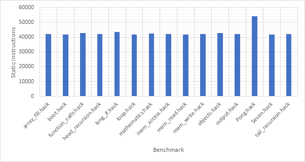
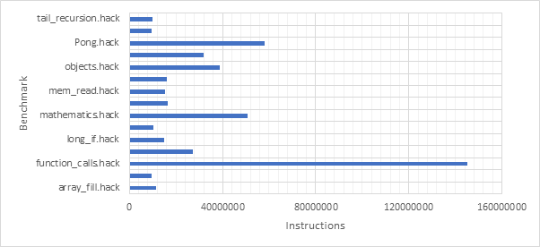
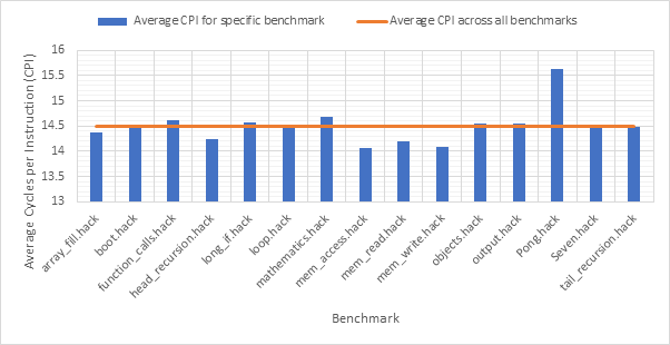
Before exploring any of the optimised configurations, it makes sense to take a look at the base configuration and the benchmark programs in order to gain a frame of reference. Figure 12 shows the number of dynamic instructions completed during the runtime of each of the benchmark programs. None of the optimisations explored in this project reduce the number of instructions completed by the CPU and so these numbers will hold for every optimised configuration. Figure 13 shows the CPI performance of the base configuration on each of the benchmarks. A lower CPI indicates a better performance. The red line shows the average CPI performance across all of the benchmarks. This then, approximately 14.5, is the number to beat.

Pipelines

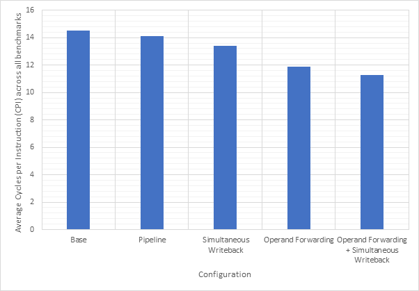
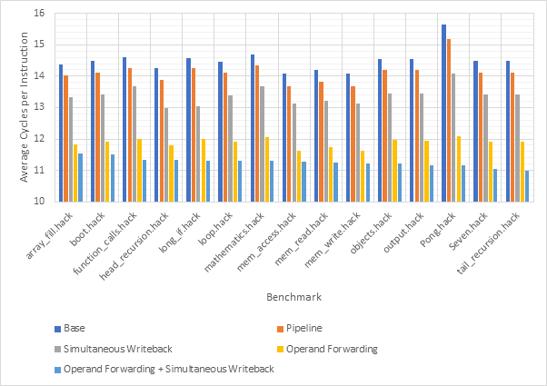
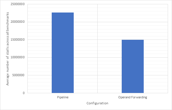
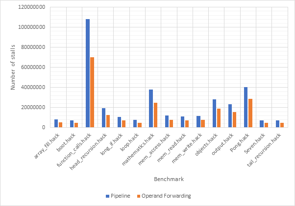
Figure 14 shows the average CPI across all 15 benchmarks for the base configuration, pipelined configuration, pipeline w/ simultaneous writeback, pipeline w/ operand forwarding and pipeline w/ simultaneous writeback and operand forwarding. Simultaneous writeback and operand forwarding are both pipeline forwarding techniques. We can see that enabling pipelining only offers a fairly paltry 2.5% performance improvement. This is likely because the pipeline spends a significant number of cycles stalled waiting for the execute or writeback stage to conclude. Both pipeline forwarding techniques help to alleviate this. The simultaneous writeback technique enables the jump sub-stage to occur at the same time as the writeback stage, effectively reducing the number of cycles required to complete the execute stage for instructions that include a jump. Whilst this only affects a relatively small number of instructions, this optimisation offers a further 5% performance improvement over the pipeline configuration and 8% improvement over the base configuration. The operand forwarding technique directly reduces the number of stalls by eliminating the need to wait for the writeback unit by enabling the operand fetch stage to retrieve operands directly from the writeback unit. This would affect a larger number of instructions than the simultaneous writeback optimisation and this results in a much larger performance improvement of 16% over the pipelined configuration and 18% over the base configuration. Since these optimisations target different areas of the CPU, they synergise well and enabling them both offers a 20% improvement over the pipelined configuration and a 22% improvement over the base configuration. Figure 15 shows the same information, but individually for each benchmark, rather than an average. Figure 16 shows the improvement in the average number of stalls across all benchmarks after enabling operand forwarding, whilst Figure 17 shows this for each benchmark individually. These graphs show that the CPI performance improvement achieved when enabling operand forwarding is due to the substantial reduction in the number of stalls.

Branch Prediction

Outcome Prediction

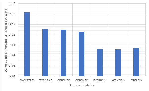
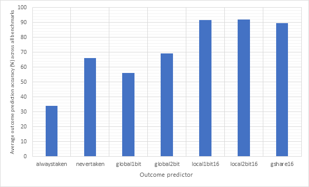
Figure 18 shows the average CPI performance of all configurations utilising each of the 7 outcome predictors. This data includes every target predictor and so may be somewhat skewed in the case that an outcome prediction is correct but the target prediction is wrong. For predictors that have a size parameter (local1bit, local2bit and gshare), this data also includes every size. Figure 19 shows the same configurations, but considers outcome prediction accuracy instead of CPI. These two graphs are highly and inversely correlated. A high prediction accuracy results in a lower CPI. Note the y-axis scale on the CPI graph - none of these strategies are having a large influence on the overall performance of the system.

Never taken is effectively the strategy taken by non-branch prediction-enabled pipelined configurations and so even though never taken is correct in around 70% of cases, it only derives a performance advantage when dealing with unconditional jumps. Conversely, the always taken strategy would derive a performance improvement when both outcome and target are correctly predicted, however due to the low accuracy of this predictor, it results in degraded performance. Neither the global1bit or global2bit strategies are able to exhibit a performance improvement over the (pipelined) nevertaken configuration suggesting that jumps in the benchmark programs are not highly correlated globally. The local1bit, local2bit and gshare strategies all achieve similar performance with the gshare strategy achieving a slightly lower performance and accuracy then the local2bit predictor. This suggests that jumps in the branch programs are more locally correlated then they are globally.

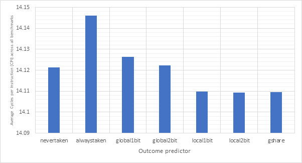
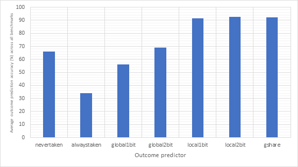
Figure 20 compares the performance of local1bit, local2bit and gshare, the highest performing strategies, by size. Figure 21 shows the same configurations but compares prediction accuracy. Here, we see a high correlation between outcome accuracy and predictor size. Unsurprisingly, larger predictors exhibit a higher accuracy and better performance, although these types of predictors would be more expensive. The graphs seem to show diminishing returns as size continues to increase, with the most pronounced improvement between sizes 8 and 16.

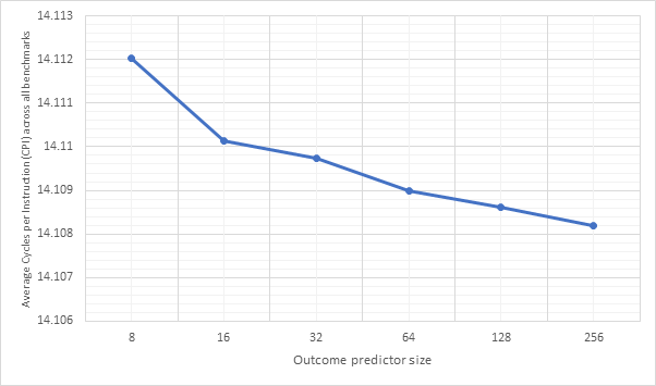
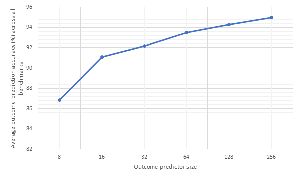
Figure 22 and Figure 23 show the CPI performance and outcome accuracy respectively for 16-line local1bit, local2bit and gshare strategies as well as the 4 unsized strategies for each benchmark individually. In this case the target predictor is set to fifo2bit256, the most accurate target predictor, to try to reduce the influence of the target predictor on these results. Here we can see once again that the 3 sized strategies outclass the other strategies and once again local2bit consistently outperforms the gshare strategy. The only exception to this is the Pong benchmark, perhaps showing that real-world benchmarks are more globally correlated then the synthetic benchmarks used in this project.

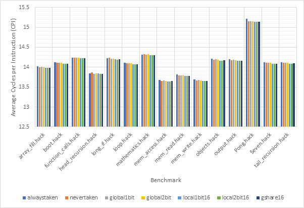
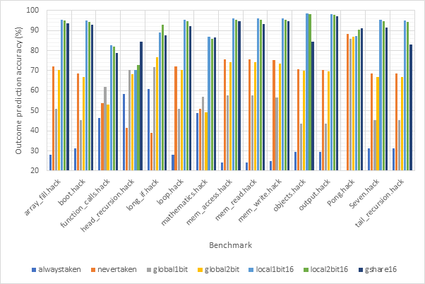
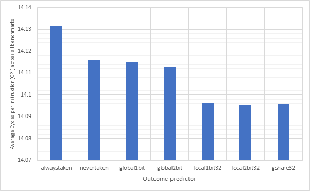
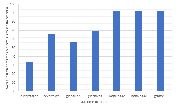
Figure 24 and Figure 25 are similar to the previous two graphs, but show averages across all of the benchmarks. Meanwhile, Figure 26 and Figure 27 show the same information, but for 32-line sized predictors. Here we can see that local1bit, local2bit and gshare remain the strongest predictors, however the performance improvements from 16-line to 32-line are fairly negligible with only a 0.003% CPI and 0.6% accuracy improvement between the 16-line and 32-line local2bit strategies, suggesting 16 may be a sweet spot.

Target Prediction

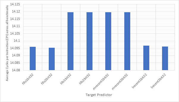
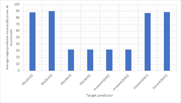
Figure 28 and Figure 29 compare the CPI performance and target prediction accuracy for each of the 2 types (1-bit and 2-bit) and the 4 eviction policies across all benchmarks. Here, we can see that CPI performance and target prediction accuracy are highly and inversely correlated. We can also see that the fifo and lrecent policies have similar performance to each other, as do the lifo and mrecent strategies. This is likely because both fifo and lrecent look to evict less recently used items, whilst lifo and mrecent evict more recently used items. Fifo and lrecent dramatically outperform lifo and mrecent in terms of accuracy, although all the CPI scores are fairly similar indicating that branch prediction does not have a major impact on CPI. The type of the predictor does not seem to have much of an impact, with 2-bit predictors consistently outperforming 1-bit predictors, but not by much. Therefore, the additional complexity of a 2-bit predictor may not be worthwhile.

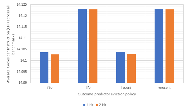
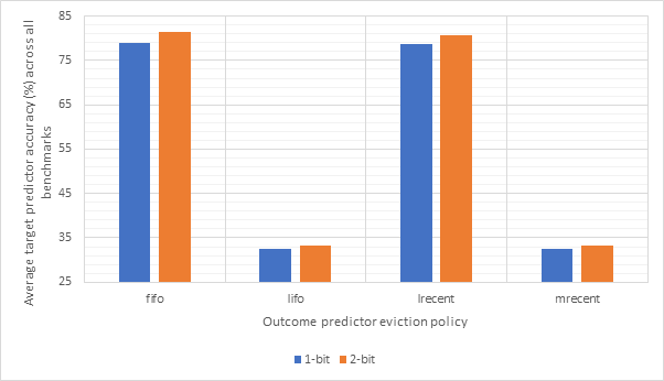
Figure 30 and Figure 31 show the relationship between target predictor size and CPI or predictor accuracy respectively. Unsurprisingly, larger target predictors offer better performance as they are able to store information about more addresses without needing to make an eviction. The sweet spot is not as clear this time, with the most notable performance improvements between 16 and 32 and between 128 and 256. The poor performance of the 8- and 16-line predictors suggests that jumps from the same address are far apart from one another meaning that smaller predictors would evict the address before it came up again. The relative stability between 32, 64 and 128 before a much larger improvement at 256 suggests that 256 may be large enough to store most of branch addresses encountered during the benchmarks. Once again, larger predictors are more expensive.

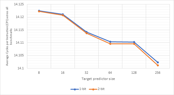
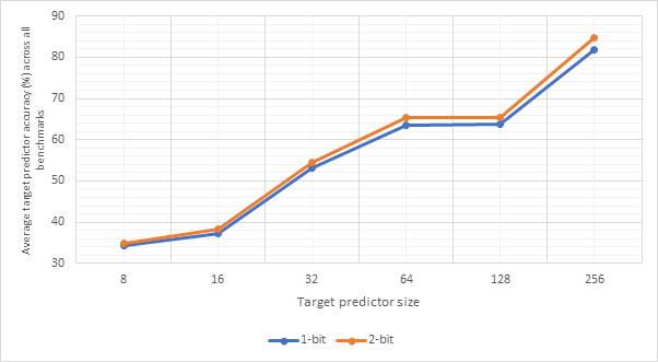
Figure 32 and Figure 33 compare the CPI performance and target prediction accuracy respectively of each of the 16-line 1-bit target predictors across each benchmark individually. The outcome predictor is set to gshare256, the highest accuracy outcome predictor encountered in this project. This is to reduce the impact outcome mispredictions on CPI figures. Figure 34 and Figure 35 show the same information for 16-line 2-bit target predictors, whilst Figure 36 and Figure 37 show this for 32-line 1-bit target predictors. Finally, Figure 38 and Figure 39 show this for 32-line 2-bit target predictors.

Consistent with previous observations, the performance of 1-bit and 2-bit predictors is very similar, potentially making the additional complexity of 2-bit predictors unwise. Also consistent with previous observations, it is clear that the fifo and lrecent eviction policies dramatically outclass the other 2 policies. When comparing 16-line and 32-line predictors, the 32-line predictors have much better accuracy scores, particularly when looking at the lifo and mrecent eviction policies.

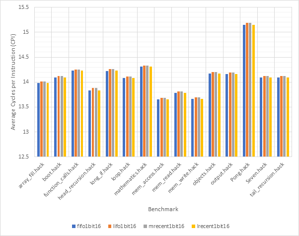
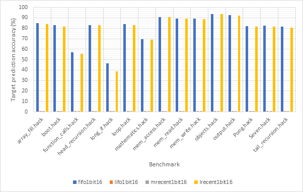
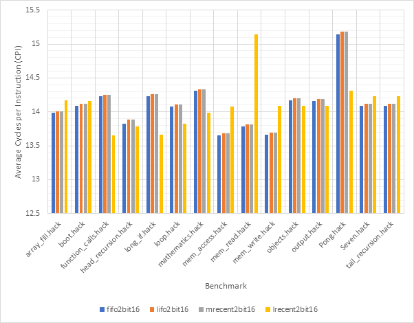
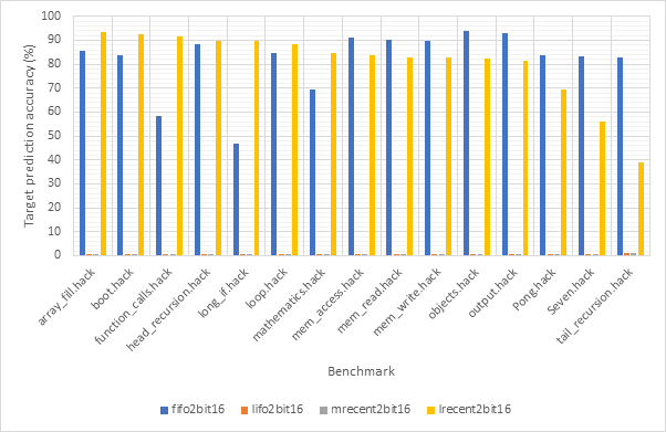
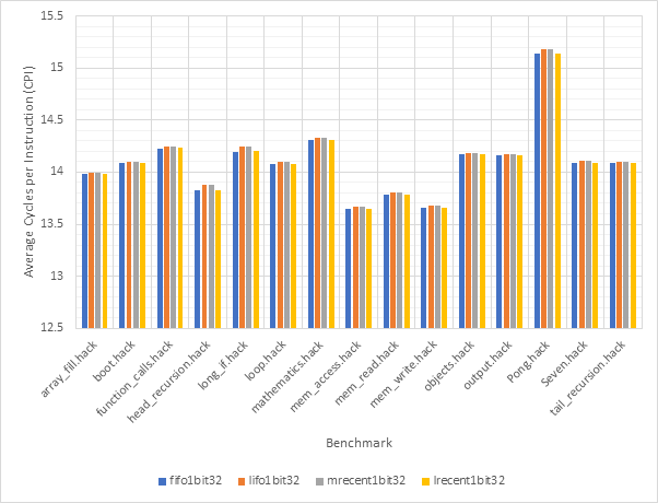
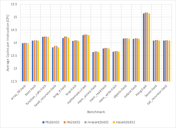
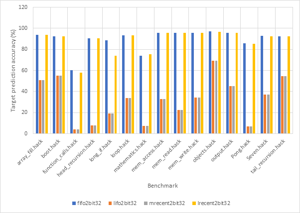
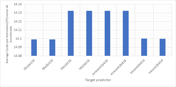
Figure 40 and Figure 41 compare the average CPI and target prediction accuracy respectively of all 16-line target predictors (both 1-bit and 2-bit) across all benchmarks using the gshare256 outcome predictor. Figure 42 and Figure 43 show the same information for 32-line target predictors. Once again, the comparatively poor performance of the lifo and mrecent strategies are highlighted, although performance does improve for the 32-line version. The fifo and lrecent policies demonstrate similar performance again and since the lrecent strategy is more complex, it is likely not worth the additional expense. The same argument can be made for 1-bit predictors over 2-bit models, the performance gain may not be large enough to worth the extra expense.

Branch Prediction

With both the target and outcome components of branch prediction now explored in detail, it’s time to take a look at branch prediction in general. Figure 44 and Figure 45 show the average CPI and branch prediction accuracy respectively for each combination of 16-line target and outcome predictors. Figure 46 and Figure 47 show the same information for 32-line target and outcome predictors. These graphs do not include the lifo or mrecent target prediction eviction policies as the poor performance of these policies excludes them from further consideration. Here we can see that within a specified size, the selection of target predictor does not make much of a difference to the performance, however the 32-line predictors do offer significantly improved accuracy scores. The selection of outcome predictor has a larger influence on results and local2bit and gshare show themselves to be the best outcome predictors once more.

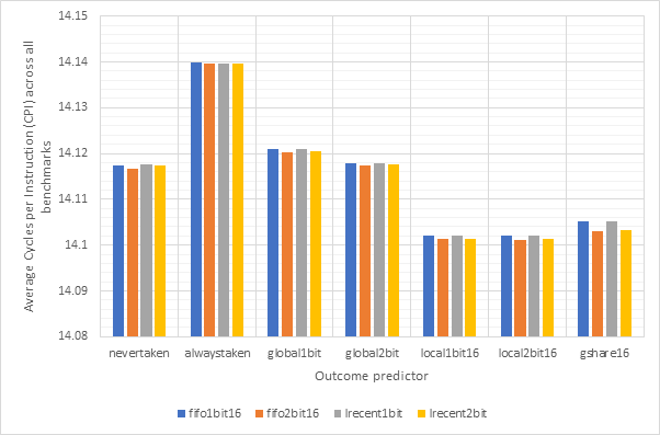
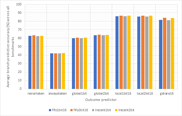
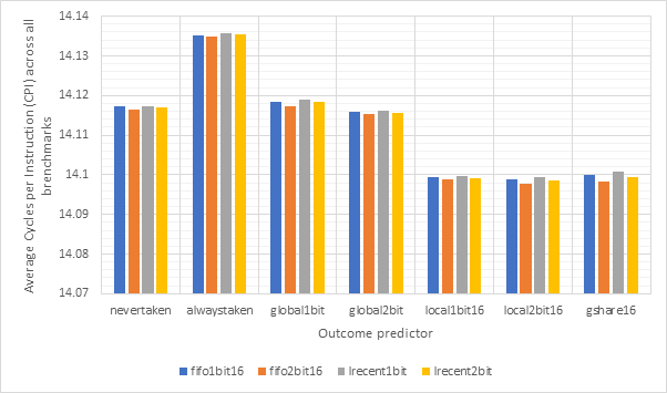
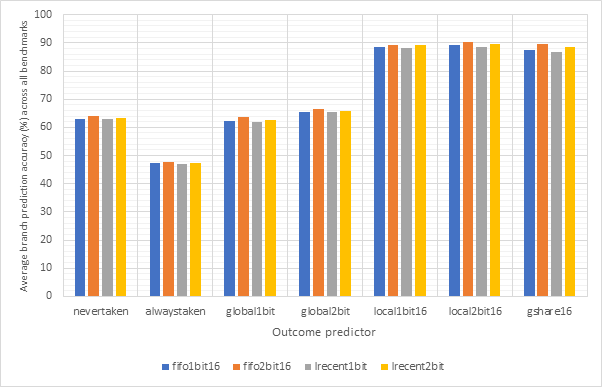
Figure 48 and Figure 49 show the average CPI and branch prediction accuracy respectively of 4 configurations for each benchmark individually. The configurations are no predictor, always taken with fifo2bit16, gshare16 with fifo2bit16 and gshare32 with fifo2bit32. Here, the two gshare-based predictors show themselves to be the best option, with the 32-line variant offering a slight performance edge over the 16-line variant. Previous observations suggested that there gshare32 did not offer much of a performance advantage over gshare32 and so these gains are likely due to the improvements offered by fifo2bit32 over fifo2bit16. Therefore, a hybrid approach of 16-line outcome predictors and 32-line target predictors may be the way to go.

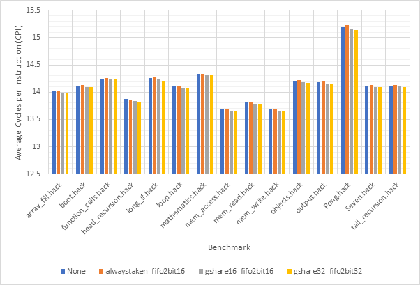
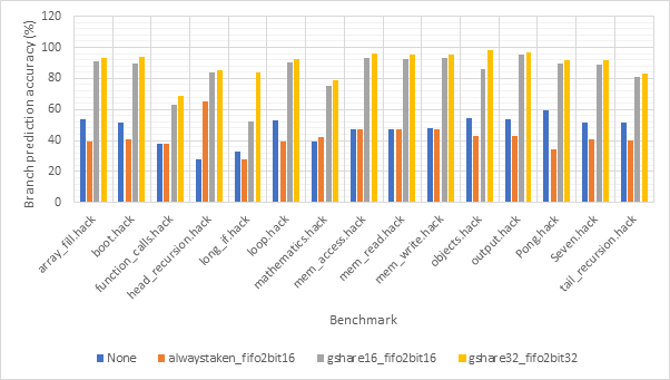
Figure 50 shows the relationship between branch prediction accuracy and average CPI performance for the 4 branch prediction configurations discussed above. This graph clearly shows the high negative correlation between branch prediction accuracy and CPI.

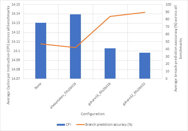
The reason that higher branch prediction accuracy leads to better CPI performance is that a successful branch prediction replaces the need for a pipeline flush with a half-flush. Half-flushes only affect the fetch unit and therefore do not impose as much of a cycle penalty. Figure 51 shows the number of flushes per benchmark for each of the branch prediction configurations. This graph clearly shows that there are less pipeline flushes for the branch prediction configurations that have higher branch prediction accuracies and lower average CPI scores. Figure 52 shows the same information but average over all of the benchmarks. It also shows the number of half-flushes.

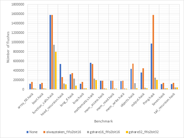
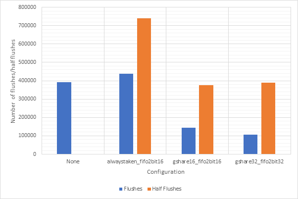
Memory Caches

Figure 53 and Figure 54 show the Average CPI performance and cache hit rate respectively for each of the cache types averaged across all sizes, eviction policies and benchmarks. Here we can see that the use of any cache, even the lowest performing static cache, dramatically improves the CPI performance of the system. This shows the memory performance is the biggest bottleneck of the system. By comparing the CPI and hit rate graphs we can see that there is a strong negative correlation between CPI and hit rate, which is unsurprising since memory caches only offer a performance improvement when accessing cached addresses. Of the four memory caches shown in this graph, direct mapped caches, fully associative caches and set associative caches all offer similar performance, although the best performance is shown by the direct mapped cache. This is likely to be misleading however, since fully associative and set associative caches make use of eviction policies and a poor eviction policy could skew the results.

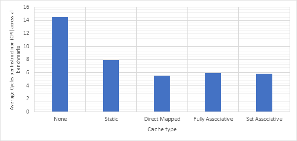
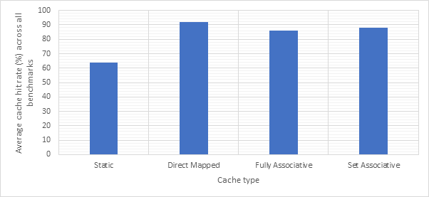
Figure 55 and Figure 56 show the average CPI and cache hit rate respectively for each of the eviction policies. These numbers are only for caches that require an eviction policy and are averaged across all benchmarks and sizes. As before, average CPI and cache hit rate are strongly negatively correlated. Just like the target predictors, fifo and lrecent offer the best performance, whilst lifo and mrecent offer poorer performance. Both fifo and lrecent offer average hit rates approaching 100%.

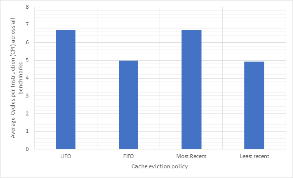
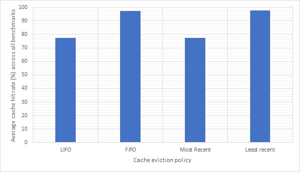
Figure 57 and Figure 58 plot the average CPI and cache hit rate respectively for each cache size across all benchmarks, types and eviction policies. Again, the CPI and hit rate charts are strongly negatively correlated. Here we can see that the performance of the memory cache improves the larger it is. This is because the cache is then able to hold a larger number of addresses.

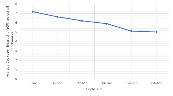
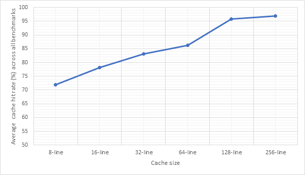
Figure 59 and Figure 60 show the average CPI performance and cache hit rate for each combination of cache type and eviction policy for 16-line caches. Figure 61 and Figure 62 show the same information for 32-line caches. Static and direct mapped caches do not use eviction policies and so these have no bearing on performance. Once again, these charts make it clear that fifo and lrecent dramatically outperform lifo and mrecent. It’s also noteworthy how small the performance improvements for the 32-line caches over the 16-line caches are. Finally, we can see that the performance of the 2-way, 4-way and 8-way set associative caches and the fully associative cache is very similar and therefore caches more complex than the 2-way set associative cache are unlikely to be worthwhile. That said, the 2-way set associative cache does offer a large performance improvement over a direct mapped cache and this is likely to be due to smaller number of conflicts.

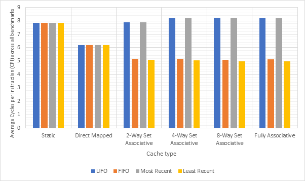
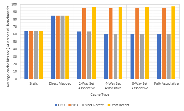
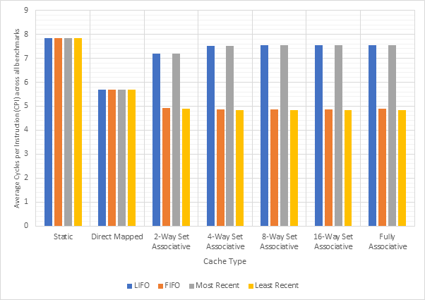
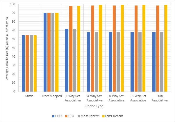
Figure 63, Figure 64, Figure 65 and Figure 66 show the same information as the last 4 graphs, albeit on a per benchmark basis instead of averaged. The 4-way, 8-way and 16-way variants have not been included due to their similarity with the 2-way and fully associative variants.

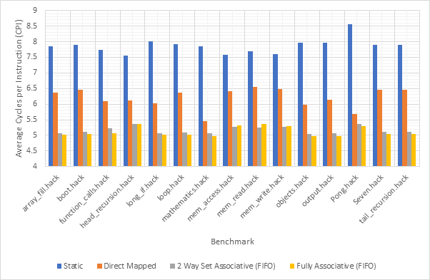
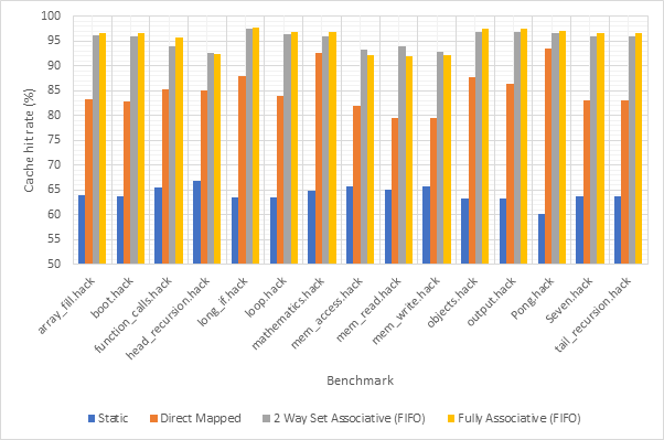
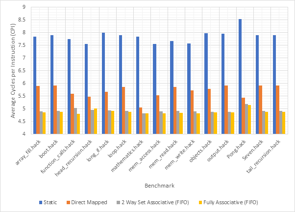
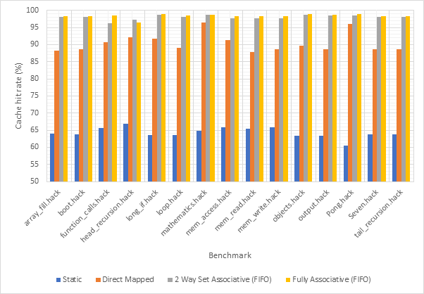
Select Configurations

Finally, a number of manually selected configurations are compared. The configurations were influenced by lessons learned during the previous three explorations. The specifics of each of the configurations are listed below:

Config A: Base configuration

Config B: Pipelined control unit

Config C: Pipelined control unit w/ pipeline forwarding

Config D: Pipelined control unit w/ gshare16_fifo2bit32

Config E: Pipelined control unit w/ gshare16_fifo2bit32 + pipeline forwarding

Config F: Pipelined control unit w/ n_way_set_associative_2_16_fifo

Config G: Pipelined control unit w/ n_way_set_associative_2_16_fifo + pipeline forwarding

Config H: Pipelined control unit w/ gshare16_fifo2bit32 + n_way_set_associative_2_16_fifo + pipeline forwarding

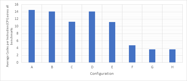
Figure 67 compares the CPI performance of each of the configurations averaged across all benchmarks. Meanwhile Figure 68 to Figure 75 show the CPI performance of each of the configurations on each of the benchmarks. Unsurprisingly, performance improves as more optimisations are enabled. When comparing B and D we can see that enabling branch target prediction, even when experiencing a high accuracy, does not have much of an impact on the CPI performance. By comparing C and E however, we can see that branch prediction has more of an impact when pipeline forwarding is enabled, although the impact is still fairly low compared to other optimisations. In contrast to this, enabling a memory cache (F) results in a massive performance improvement, more than halving the CPI. Config H represents the most highly optimised configuration explored here. It was selected as it can achieve an excellent CPI score, however the components chosen also offer value for money. Whilst other choices, such as a larger cache or target predictor or a fully associative cache could have offered better performance, these components would be substantially more expensive or complex and would be unlikely to offer particularly dramatic performance improvements over those seen in H.

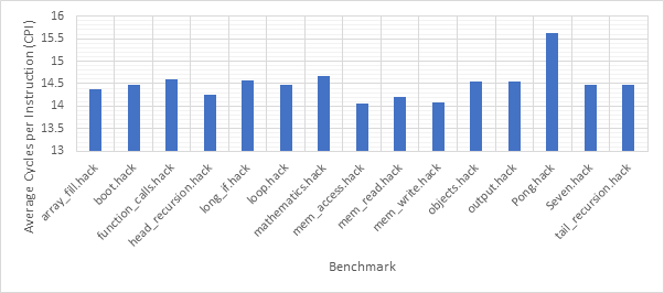
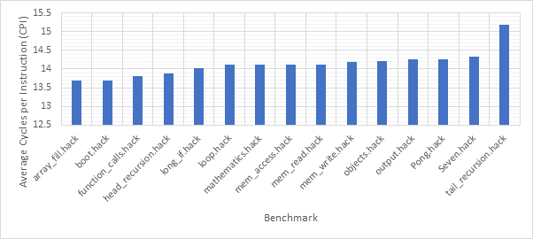
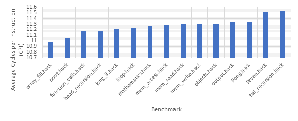
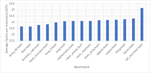
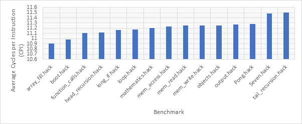
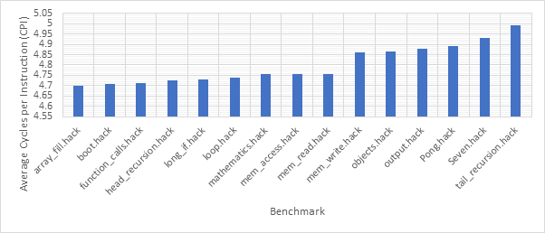
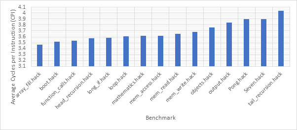
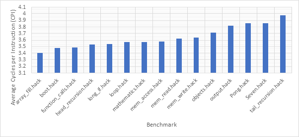
Evaluation

This project was able to gather a substantial volume of data, with the capability to gather substantially more data given sufficient time and/or hardware. The data gathered enabled a detailed exploration of 5 major modern hardware optimisation techniques: pipelining, (two variants of) pipeline forwarding, memory caches, branch outcome prediction and branch target prediction. The application of statistical analysis and data visualisations enabled the performance impact of each of these optimisations to be examined and compared. For memory caches and branch prediction, the data also enabled an analysis and comparison of different types of cache, target predictor and outcome predictor. In addition to this, the impact and optimal values for parameters such as size and eviction policy was evaluated.

This project was able to graphically demonstrate the underlying causes for many of the performance improvements. It was shown that performance improvements from operand forwarding are due to a reduced number of pipeline stalls. The project was able to demonstrate that the performance improvements derived from branch target and outcome prediction are directly linked to the prediction accuracies for these components. The project was then able to show that a high branch prediction accuracy leads to a reduction in the number of pipeline flushes. Both of these factors could be highly correlated to performance improvements. Similarly, it was able to show that performance improvements as a result of memory caches are driven by the cache hit rate.

For the Hack platform, this project was able to show that memory caching would be the single most impactful optimisation, able to improve performance by a factor of 3. The second most impactful optimisation would be pipeline forwarding, which could not function without the pipelining optimisation.  The least impactful optimisation is branch prediction, which was only able to improve performance slightly. These observations could be very useful to future hardware designers when determining which optimisation to prioritise. However, the proportional impact of each of the optimisations may not translate well to other architectures. Branch prediction, for example, may have a much greater impact for other architectures. This could be, for example, because that architecture supports direct branches.

This project culminated in configuration H, the most highly optimised version of the Hack platform. This configuration made use of every optimisation explored in the project. The memory cache selected for the configuration was a 16-line 2-way set associative cache, using a FIFO eviction policy. The FIFO eviction policy was selected as it is simpler but offers similar performance to the least recent policy, whilst offering much better performance than the most recent or LIFO policies. A 2-way set associative cache was chosen as it offers dramatic performance improvements over a direct mapped cache, whilst offering similar performance to set associative caches with a larger number of ways, or the fully associative cache. All of these alternatives are more complex and expensive. The 16-line variant was selected as the step up in performance between 8 lines and 16 lines was most pronounced and larger caches did not offer substantially higher performance but would be more expensive. The outcome predictor selected was 16-line gshare. Gshare was chosen despite offering slightly lower performance than local2bit predictors because it is able to leverage global information and showed a slight performance improvement in the Pong benchmark, which is the most “realistic” benchmark. A size of 16 was chosen as further increases in size did not dramatically increase the performance of the predictor. The target predictor chosen was a 32-line fifo2bit predictor. The FIFO eviction policy was chosen for the same reasons it was chosen for the memory cache. Despite the 2-bit variant offering only slight performance improvements, it was selected as an additional bit does not introduce significantly more complexity into the hardware design. A 32-line variant was selected as there were dramatic improvements between the 16- and 32-line variants. Whilst these predictors continued to improve in performance as more lines were added, these additional lines come at an increasing cost, as the number of lines must double each time. Since the Hack platform has a relatively small amount of program memory, 32-line target predictors are the largest that can be justified. Configuration H is able to offer 4 times better performance than the base model which is a dramatic improvement.

This project was not able to quantify the cost or complexity of the optimisations proposed. For example, fully associative caches would be substantially more complex and expensive than direct mapped caches, although these factors have been addressed in the text, the simulations did not account for them. If these costs could be quantified it would provide more rigour to these arguments. One way to quantify the costs could be to present a digital circuit implementing the relevant logic and using the number of primitive logic gates required to build the circuit as a complexity metric.

This project was not able to account for the additional time it might take for a fully associative cache to lookup a value in the cache. This additional lookup time would come as a result of the increased complexity of implementing full associativity. The simulations used in this project do not account for this – even though the fully associative cache has a better accuracy, it may perform worse than a direct mapped cache due to a longer look up time.

One final criticism of the project is that the simultaneous writeback optimisation requires the introduction of a second memory unit. This is because it becomes possible for a read and write operation to occur at the same time. The introduction of a second memory unit obviously introduces additional costs, complexity and space requirements to the CPU. These additional factors are not accounted for during simulation. Additionally, the introduction of dedicated read/write units results in two separate memory caches (again increasing complexity). The impact of separate memory caches was not evaluated by this project. A possible improved approach could be to introduce a queuing system within the memory unit such that only one unit is required.

Future Work

Whilst exploring the results, it was noted that branch prediction has a low impact on the performance of the system. In the future, it would be interesting to evaluate whether the branch prediction components could be moved into the fetch unit and therefore predictions could be made earlier in the pipeline, eliminating the need for half flushes.

Although this project has been able to look at some of the hardest hitting optimisations, such as memory caches, there are still many more optimisations that could be examined. Unfortunately, due to time constraints, not all of them could be explored in this project. However, if there was more time, there are a number of very important optimisations which would be very valuable additions to this project.

Speculative execution and out-of-order execution are two optimisation techniques that are utilised heavily in modern CPUs. It would have been valuable to evaluate how these major optimisation packages compare with the optimisations already explored in this project. It would also be worth investigating how CPU performance could be improved by adding additional functional units, such as having two ALUs.

Another interesting direction for the project would be to further investigate parallelisation. Whilst this has already been touched upon through the use of pipelining and the simultaneous writeback optimisation, there is a lot more that could be done. The addition of vector functional units enabling SIMD would have been one particularly compelling area. An alternative approach could have been to include two or more complete CPUs and move into the multi-core domain. Both of these optimisations would likely require new instructions to be added to the system, which would have required changes at every level of the software hierarchy.

It would have been fascinating to evaluate adding multiply and divide instructions and dedicated functional units for these operations. The current implementations for multiple and divide are very slow and inefficient, requiring repeated addition or subtraction.

One area of improvement for the Hack platform that would be intriguing to explore, but is not necessarily related to hardware optimisation would be to enable the system to modify the ROM during runtime. This would move the system closer to modern computing systems that are able to download new programs and run them without any changes to the hardware. This would also make “self-hosting” a possibility, meaning that developers could write, compile and run code directly on the Hack platform without needing access to another machine. In addition to physical hardware changes, all of these ideas would require the operating system to play a much larger role.

Improving the operating system would also be a highly interesting and educational task. As mentioned previously, the current operating system is closer to a standard library than an operating system. Modifying the operating system such that it could support tasks as described above would be a complex undertaking. The operating system would need to be capable of loading a new program without rebooting. It would also be interesting to add other modern features, such as multiple users or multi-tasking to the operating system.

Conclusion

After providing an overview of Nissan and Schocken’s Hack platform, this project has explained what CPU optimisations are and why they are needed. A brief study of old and modern CPU architectures enabled a realistic cycles per instruction schedule to be defined. Three generations of CPU simulator were developed, culminating in a simulator offering high performance and an elegant programmatic format for defining optimisations. 15 benchmarks were defined, 2 of which are “real-world” benchmarks taken from the book and 13 “synthetic” micro benchmarks testing various aspects of the CPU were developed as part of this project. This was followed by a detailed description of 5 modern CPU optimisation techniques. A toolkit for running batches of simulations was then developed in python. This toolkit was used to run and generate results for around 20,000 different configurations – where each configuration featured a different combination of optimisations and benchmark program. A graphical and textual deep dive of these results was then conducted, culminating in an insightful evaluation of the results.

This project has been able to show that the most impactful CPU optimisation is memory caching. This finding can be explained by the fact that accessing memory is one of the most fundamental operations that a CPU performs. Despite this, advances in memory technology have not been able to keep pace with advances in processor technology. This has resulted in a situation where CPU performance is often bottlenecked by memory performance. In this context, it is easy to see why offering the CPU a bank of faster memory could offer dramatic performance gains.

This project has also been able to show that pipelining and pipeline forwarding offer a valuable set of tools for increasing the instruction throughput of a CPU. These techniques enable a degree of instruction-level parallelism, which can improve performance by enabling a CPU to perform multiple tasks simultaneously. Pipeline forwarding further increases the level of parallelism by allowing the CPU to process branch instructions and perform memory writeback simultaneously, as well as enabling the fetching of operands directly from the writeback unit, rather than waiting for these operands to be written back to memory. These techniques offer a moderate impact on the performance of the system.

Despite being able to demonstrate a highly accurate branch prediction subsystem, consisting of outcome and target predictors, this project was not able to derive a particularly impactful performance improvement from branch prediction. However, it is this author’s opinion that greater performance gains could be derived on alternative architectures.

Configuration H, produced by this project, was able to offer a significant 4 times performance improvement over the base configuration. This is a substantial performance improvement and shows that CPU optimisation techniques are valuable and effective. As other avenues for deriving performance gains, such as increasing clock speed, begin to reach their limits, developing and improving CPU optimisations will become increasingly important.

The contribution of this project has been to compare and contrast some of the most important modern CPU optimisations. As well as helping readers to understand how these optimisations work and why they are needed, this report presents a simple hardware architecture that provides the ideal test bench for testing CPU optimisations. The simulation software developed in this project provides an environment for gaining hands-on experience interacting with the system and gathering results in an automated fashion. The use of a modular design makes it easy for anyone to develop a new optimisation for the platform. This report outlines which optimisations have the greatest impact on performance and uses data visualisation to present these results to the reader, which can act as a set of guidelines to hardware designers.

References

Appendix A: Links

Nand2Tetris implementation: https://git.jbm.fyi/jbm/Nand2Tetris

1^st Generation Simulator: https://git.jbm.fyi/jbm/Hack_simulator

2^nd Generation Simulator: https://git.jbm.fyi/jbm/Hack_sim2

3^rd Generation Simulator: https://git.jbm.fyi/jbm/Hacksim3

Hack toolchain: https://git.jbm.fyi/jbm/Hack_toolchain

Benchmarks (and toolkit): https://git.jbm.fyi/jbm/Hack_benchmarks

Appendix B: Hardware Implementation

This section will present and explain an implementation of the Hack architecture based on the Nand2Tetris course [1]. This implementation will serve as both a reference Hack implementation and as a base model to be optimised later in the project. Additionally, this section will provide the reader with an understanding of the construction and capabilities of the system. The only components required to construct the computer are NAND gates and Data Flip-Flops (DFFs).

Primitive Logic Gates

Fundamentally, a computer is nothing but a collection of logic gates arranged in such a way as to facilitate the execution of a program. Logic gates are units that take a number of binary inputs and produce a number of binary outputs based on the input value(s). There are four primitive logic gates: NOT, AND, OR and XOR. NOT gates take one input and produce one output that is the opposite of the input (1 if the input is 0 and vice versa). The remaining gates take two inputs and produce one output. AND produces 1 if both inputs are 1, OR produces 1 if at least one input is 1 and XOR produces 1 if exactly one of the inputs is 1. In addition to these primitive gates, there are three negated versions of the primitives: NAND, NOR and NXOR. These are simply a AND, OR or XOR gate who’s output is negated. Conveniently, any of the other gates mentioned here can be constructed from a collection of NAND gates. This makes them an ideal choice as a basic building block. Figure 76 – Figure 79 show how the four primitive logic gates can be derived from NAND gates.

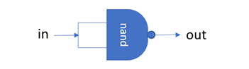
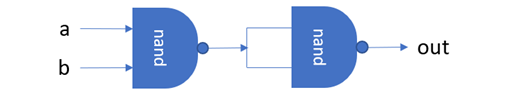
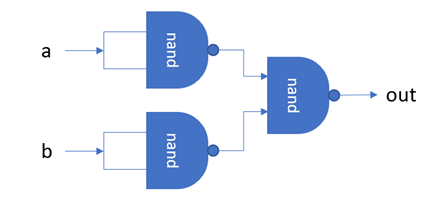
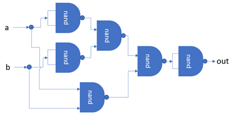
Multi-bit Primitive Logic Gates

As the system under construction is 16-bit, it will require 3 multi-bit versions of these primitive logic gates. The first is an 8-way OR gate. This gate takes an 8-bit input and generates a 1-bit output that is the result of ORing all of the input bits together. This means the gate will return 1 if any of the input bits are 1, or 0 otherwise. Figure 80 derives the 8-way OR gate from primitive OR gates.

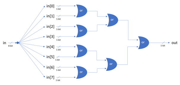
Next, the system requires 16-bit versions of the NOT and AND gates. These are both bitwise gates meaning that they apply the logical operation to each bit of the input(s) independently. In the case of the 16-bit bitwise NOT gate, each bit of the input is negated. The 16-bit bitwise AND gate takes two 16-bit inputs and returns a 16-bit output where each bit is the result of ANDing together the corresponding bits in both inputs; i.e. out[0] = a[0] AND b[0]…out[n] = a[n] AND b[n]. Both gates are derived from their respective primitive gates in Figure 81 and Figure 82 shown below.

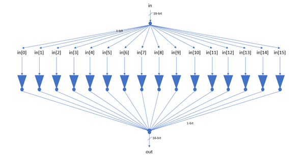
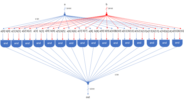
Multiplexer and Demultiplexers

Multiplexer and demultiplexers are heavily relied upon during the construction of the system. Multiplexers take two input signals and send one of them to the output. The signal that is outputted is determined by a third input. Demultiplexers perform the opposite operation, they take one input and have two output channels. A second input controls which output channel the input should be sent to. Figure 83 and Figure 84 show how multiplexers and demultiplexers respectively can be derived from primitive logic gates.

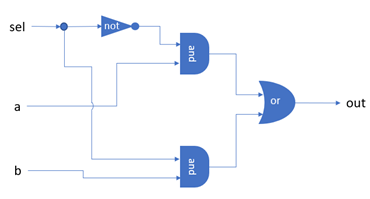
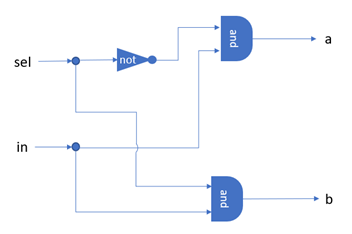
Four and eight-way demultiplexers can be easily derived from basic demultiplexers as shown in Figure 85 and Figure 86.

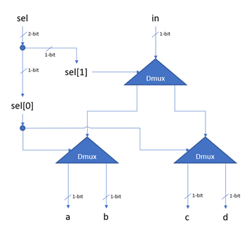
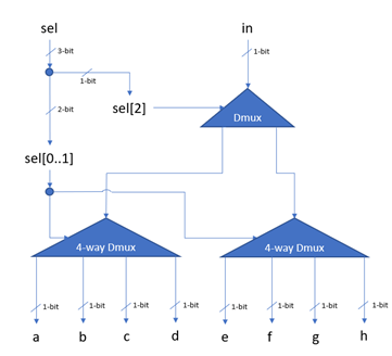
16-bit versions of multiplexers are required so that 16-bit buses can be routed round the system. These can be derived from basic multiplexers, shown in Figure 87.

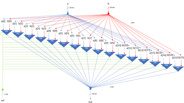
Again, four and eight way 16-bit multiplexers can be derived from 16-bit multiplexers as shown in Figure 88 and Figure 89.

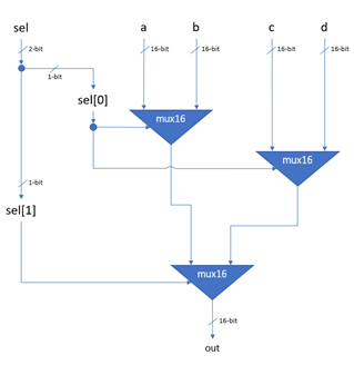
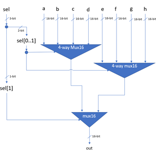
Binary Arithmetic

The Hack system uses 16-bit two’s complement binary to represent integers where the left most bit is the Most Significant Bit (MSB). Two’s complement is a scheme used to represent signed integers in binary where the MSB retains its magnitude but becomes negative. This will mean that the largest positive number will be represented as 0 followed by 1s, the largest negative number will be represented as 1 followed by 0s, -1 would be represented by every bit being 1 and 0 would be represented by every bit being 0. The MSB for any negative number will always be 1. Two complement is a convenient representation as maths operations such as addition still work as normal without any special considerations for signage.

If integers can be represented as a series of bits (1s and 0s) on a wire, then circuits that can perform arithmetic operations can be built. The simplest of these is a half adder which takes two 1-bit numbers and outputs the sum of the two numbers and indicates if there is a carry. As there are only two inputs to the half adder, it is not able to account for any carry from previous additions. This problem is solved by the full adder, which has a third input enabling it to forward any carry bits. The full adder is derived from primitive logic gates in Figure 90.

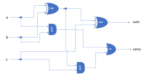
Once again, in order to deal with 16-bit numbers, the Hack system requires a 16-bit version of the full adder. This is shown in Figure 91 below.

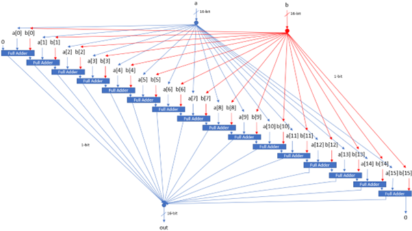
Arithmetic Logic Unit (ALU)

An Arithmetic Logic Unit or ALU is a digital circuit that can perform arithmetical or logical operations on integer inputs. Traditionally, the ALU is the centrepiece of a computer processor, however modern processors may have multiple ALUs or may consider other units (such as a Floating-Point Unit) to be of co-equal importance.

The Hack architecture, with its focus on simplicity, dictates that the ALU should be as simple as possible, implementing only the most essential operations and leaving the rest to be implemented in software. The Hack ALU takes two 16-bit integers x and y as input and produces one 16-bit integer out as output. The operation performed on the two inputs is determined by six 1-bit control inputs and the ALU also has two 1-bit status outputs.

The six control inputs are designated zx, zy, nx, ny, f and no. Zx and zy are used to zero the x and y inputs respectively. Nx and ny are used to negate the x and y inputs respectively. F is used to specify the operation, if set to 0 a bitwise AND operation will be performed on the inputs and if set to 1 the inputs will be added together. Finally, no is used to negate the output. There are 64 possible combinations of control inputs each of which affects a different function. However, only 18 of these are of interest and these are shown in Table 6. Symbols !, & and | represent bitwise NOT, AND and OR respectively.

Table 6 ALU operations based on Figure 2.6 of The Elements of Computing Systems [1].

The two status outputs are designated ng and zr. Ng is set to 1 if the output is negative, whilst zr is set to 1 if the output is equal to zero.

An implementation of the Hack ALU from logic gates previously derived in this section is shown in Figure 92.

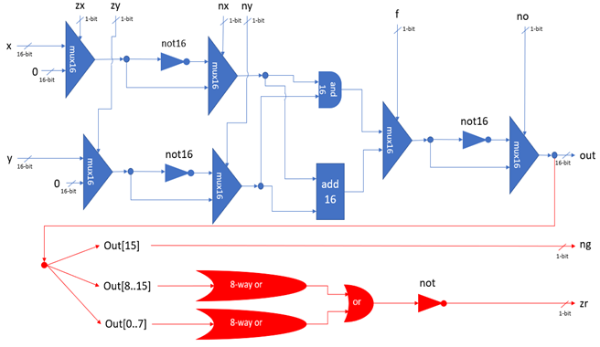
Memory Chips

All the chips discussed up to this point in this section have been combinational circuits, named so because their outputs depend entirely on the combination of their inputs. Whilst these chips are able to perform a wide variety of useful functions, they are not able to maintain state. Computers must be able to maintain state and this is where memory chips which employ sequential logic come in.

The act of remembering something implies the concept of time. Therefore, computers must have a method of keeping time. For most computers, an oscillator which alternates between two states, 1 and 0, serves as the clock. The time between the first state starting and the second state ending is called a cycle and each cycle models one time unit. The computer can then be synchronised by broadcasting the clock signal to every sequential chip in the system.

The implications of sequential logic, including clocks and synchronisation, can be abstracted away into a single chip – the Data Flip-Flop (DFF). DFFs are the second elementary building block needed for the system and have one input and one output. In addition to these, the DFF must be connected to the clock. The output of a DFF is its input in the previous clock cycle.

DFFs become latched at the beginning of each clock cycle. Once a DFF is latched, its output will not change until the start of the next cycle. This means that the output value of a DFF is committed at the start of each cycle. As all of the combinational logic used in the system will eventually output to a sequential element, the output of combinational circuits only matters at the start of each cycle. Therefore, as long as the length of a cycle is at least as long as the maximum propagation time within the processor, the outputs of combinational circuits can be guaranteed to be valid the start of a cycle and it doesn’t matter if the outputs of these circuits is undefined up until that point.

The most basic memory chip in the system is the bit. A bit is simply a DFF with an interface that enables a new value to be loaded into the DFF at select times. The DFF retains its value at all other times. The bit is implemented from DFFs and previously derived logic gates in Figure 93 below.

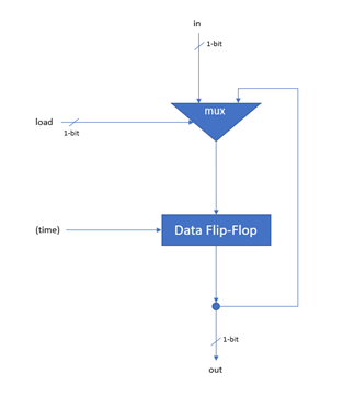
Following the pattern we are now used to, a 16-bit version of the Bit is needed and this is referred to as a register. The register is implemented in Figure 94 below.

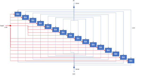
The Random Access Memory (RAM) unit of the Hack system is made up of a bank of registers along with addressing circuitry to specify which of the registers should be accessed. This is implemented through a hierarchy of memory bank chips with varying sizes: 8-bytes, 64-bytes, 512-bytes, 4-kilobytes and 16-kilobytes. An implementation of the first of these chips is shown in Figure 95 below.

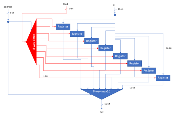
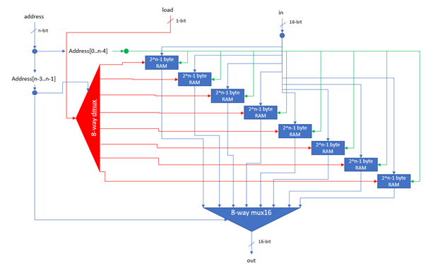
The 16K RAM unit is slightly different and its implementation is shown in Figure 97 below.

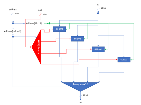
When a computer processor is executing a program, it must keep track of which instruction should be executed next. This job is done by a specialised register called the Program Counter or PC which stores the address of the next instruction to be executed. After executing an instruction, the PC is usually incremented so that the next instruction can be executed, however in some cases (namely jumps), execution may be resumed from a different address. Finally, there must be some way to reset the computer so that it restarts the execution of the program. The PC implemented in Figure 98 below will increment its value if inc is 1, will set its value to in if load is 1 and will set its value to 0 if reset is 1. In all other cases, the value of the PC will remain the same.

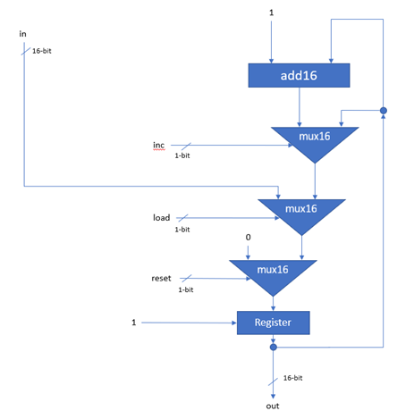
Memory Unit, ROM and Peripherals

The final RAM unit for the system is shown in Figure 99.

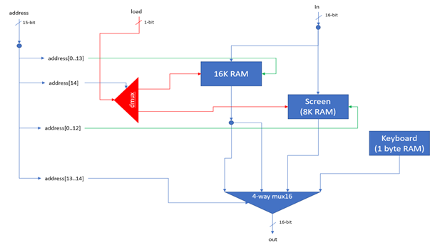
The memory unit has the same interface and looks similar to the memory bank chips defined in the previous sections. However, unlike the previous chips, there are only three underlying banks and each are of a different size. The 16K RAM chip is the same as the one defined in the previous section, however the other two chips are memory-mapped peripherals.

Memory mapping is a technique in which peripheral devices are represented to the computer by one or more bytes in the RAM. This scheme is much simpler and scalable then the alternatives.

The Hack system is equipped with a 256 (height) by 512 (width) monochrome display. This is represented by an 8K RAM chip which, from the computer’s perspective, can be used in exactly the same way as any other 8K RAM chip. However, setting any bit within this memory space will have the effect of illuminating the corresponding pixel in the display. Each row in the screen is represented by 32 consecutive 16-bit words starting at the top-left corner of the screen. The pixel at row r (from the top) and column c (from the left) is represented by the c%16 bit of the word found at Screen[r*32+c/16].

The Hack system is also equipped with a standard keyboard. This is represented by a 1-byte RAM chip (register) that can be read from in the same way as any other memory chip. It is, however, different to every other memory chip in that there is no mechanism for writing a value to the memory space. Instead, the register will be populated by the ASCII code representing whichever key happens to be held at the current time, or 0 if no key is held. Special keys are represented by the codes shown in Table 7.

Table 7 Special keyboard codes taken from Figure 5.6 of The Elements of Computing Systems [1].

Programs are supplied to the Hack system in the form of replaceable cartridges. Each cartridge contains a Read Only Memory (ROM) Chip. This is a memory chip that is similar to the previously discussed memory bank devices, however it lacks a mechanism to write new values to the registers. Each register stores a single instruction. The size of the ROM chip is 32 kilobytes, however not every program will use the entire available space.

Central Processing Unit (CPU)

All the chips needed to build a Hack Central Processing Unit (CPU) have now been defined. The Hack CPU has 3 registers: A, D and M. D is a general-purpose data register; A can be used as either a general-purpose data register or as the address register; M is a virtual register that always refers to the memory location with the address of the current value of A (M = RAM[A]).

Instructions are supplied to the CPU as a 16-bit word. We will refer to each of the bits in the instruction using the labels shown in Table 8 below.

Table 8 Instruction bit labels.

There are two types of instruction: A-instructions and C-instructions. The t-bit determines which of the two types an instruction is.

A-instructions are used to load a value into the A register. A-instructions are encoded by setting the t-bit to 0. The remaining bits (bits 1-15) form a 15-bit integer that is loaded directly into the A register. For example, the instruction 0000 0000 0000 0101, would load the value 5 into the A register.

C-instructions are encoded by setting the t-bit to 1. Neither x-bit is used by the C-instruction and so both should also be set to 1. The remaining bits then form 3 fields: Computation (comp), Destination (dest) and Jump (jump).

The comp field consists of bits 3 – 9 are is used to specify what the ALU should compute. The value contained within the D register is always used as the x-input to the ALU. The y-input could be either A or M and this is specified by setting the a-bit to 0 or 1 respectively. The remaining bits specify the control inputs to the ALU. There are 128 possible combinations of the 7 comp bits, of which only 24 are included in the Hack specification. These are shown in Table 9, note that the left-most and right-most columns show the function (and assembly mnemonic) that would be computed given the specified c-bits if the a-bit is 0 and 1 respectively. For example, the comp part (shown in bold) of the instruction 1110 0011 1000 0000 would instruct the ALU to compute D-1.

Table 9 Possible comp field values based on Figure 4.3 of The Elements of Computing Systems [1].

The dest field consists of bits 10 – 12 and specifies where the output of the ALU should be stored. If d₁ is set, the output is stored in the A register; if d₂ is set the output is stored in the D register and if d₃ is set the output is stored in the M register. One, more than one, or none of the d-bits may be set.

The jump field specifies which instruction should be executed next. There are two possibilities, either the next instruction in the program will be executed (which is the default) or execution will resume from the address stored in the A register (referred to as a jump). Which of these outcomes occurs is determined by the three j-bits and the output of the ALU. If none of the j-bits are set then no jump will occur; if j₁ is set a jump will occur if the output is negative; if j₂ is set a jump will occur if the output is equal to zero and if j₃ is set a jump will occur if the output is positive. If all three bits are set a jump will occur unconditionally. The combination of these three bits gives rise to eight possibilities as shown in

Table 10 Possible jump field values based on Figure 4.5 of The Elements of Computing Systems [1].

An implementation of the Hack CPU based on previously derived components and capable of the behaviour described above is shown in Figure 100.

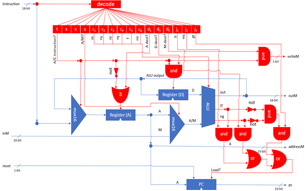
Complete System

Finally, the complete hardware implementation is shown in Figure 101.

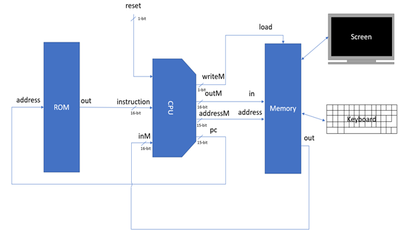
Appendix C: Software Implementation

This section contains a brief exploration of the software stack for the Hack platform, for more details see The Elements of Computing Systems [1].

Assembler

The instructions for the Hack CPU take the form of 16-bit binary integers. Understandably, humans do not find it easy to work with long lists of numbers. Luckily, the limited number of possible values for each of the three fields (comp, dest and jump) making up the instruction make it trivial to define a one-to-one mapping of mnemonics to binary encodings. Taken together, these mnemonics form a basic programming language known as Hack assembly.

Hack assembly A-instructions take the form of @constant, which simply loads the constant into the A register. On the other hand, C-instructions take the form of dest=comp;jump. The dest and jump fields are both optional but comp is compulsory. If the dest field is empty then ‘=’ may be omitted, whilst ‘;’ may be omitted if jump is empty.

The dest mnemonic may be any combination and order of the symbols ‘A’, ‘M’ and ‘D’. The result of the comp field will then be stored in each of the registers present. The possible comp mnemonics are listed in Table 9 and the possible jump mnemonics are listed in Table 10.

Note that when affecting an unconditional jump, it is conventional to use the instruction “0;JMP”. This is because the comp field is mandatory but ignored during unconditional jumps. Therefore, the convention is to have the ALU simply compute 0. Also note that there are conflicting uses of the A register. The programmer can use the A register to store a data memory address for a subsequent C-instruction involving M, or it can be used to store an instruction memory address for a subsequent instruction involving a jump. Therefore, to avoid undefined behaviour, an instruction that may cause a jump should not use the M register.

The program that translates between assembly code and binary machine instructions is called an assembler. The assembler developed for this project is written in the Rust programming language and a link to the source code can be found in Appendix A. In addition to simple translation duties, the assembler program also manages two types of symbols which makes life easier for the programmer.

The first type of symbol is a label which can be defined using the pseudo-command “(label)”. This will define a symbol referring to the address (in program memory) of the instruction immediately after the label. These labels can then be used as targets for jumps. A label can only be defined once but can be used anywhere within the program.

The second type of symbol is a variable. The assembler will assign a memory address (between 16 and 255) to each previously unencountered symbol. When the symbol is encountered again in the future, it will be translated to the previously assigned memory address. This frees the programmer from the burden of manually assigning variables to memory locations.

In addition to these user-defined symbols, there are a number of predefined symbols. First there are 16 virtual registers R0 – R15, these refer to memory locations 0 – 15. In addition to these, the symbols SP, LCL, ARG, THIS and THAT also refer to memory locations 0 – 4 (these are used in the virtual machine implementation later). Finally, the symbols SCREEN and KBD refer to the bases of the screen and keyboard memory maps at memory addresses 16384 and 24576 respectively.

One final duty of the assembler is to remove comments, which can be created by using the symbols “//” at the start of a line.

An example of a simple assembly program, which multiplies two numbers together, is shown in Figure 102.

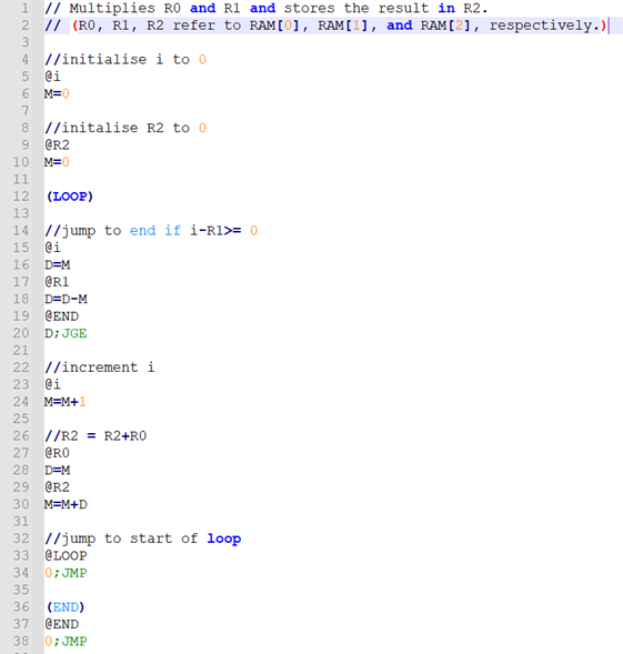
Virtual Machine (VM)

Writing programs for the system in assembly is substantially more convenient then writing them in machine code, however, for the programmer used to the bells and whistles available in modern programming languages, it still seems primitive. The next step then, is providing a compiler to enable a high-level language to be used on the Hack platform. Some compilers go down the route of translating high-level code directly to assembly, however, today it is more popular to first translate the high-level code into an intermediatory medium-level language and then later translate the intermediatory code into assembly and finally machine code. As well as allowing for abstraction, this approach has the benefit of decoupling the “front” and “back” ends: once an intermediatory code translator program has been written for a platform, any language that can compile to the intermediatory code can be run on that platform; and once a high-level to intermediatory code translation program has been written, the high-level code can run on any platform which has an intermediatory code translation implementation.

The Hack platform specifies a Stack-Based Virtual Machine (VM) that can run a specified intermediatory language called VM language. The virtual machine consists of 8 memory segments: argument, local, static, constant, this, that, pointer and temp, as well as the stack and heap. Values can be pushed onto the stack from a segment or popped from the stack into a segment using the commands push [segment] [index] and pop [segment] [index] respectively. Operations can be performed by first pushing the operands onto the stack and then calling a function or operation. In either case the operands will be popped off the stack and the result pushed onto the stack, as shown in example in Figure 103. Built in operations are add, sub, neg, eq, gt, lt and, or and not and programmers can define functions to perform other operations. Functions are defined using the syntax function [name] [numLocals] where both a name of for the function and the number of local variables within the function must be specified. Functions can be called using the syntax call [name] [numArgs] where both the name of the function to be called and the number of arguments must be specified. Programmers can also define labels using the label command which can be jumped to using goto, or conditionally jumped to using if-goto. If-goto pops the top item off the stack and if it is not zero execution resumes from the label and otherwise continues with the next instruction. Finally, functions are returned from using the return command.

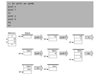
The argument and local memory segments store a functions arguments and local variables respectively. The static memory segment is shared by all functions in the current file. The this and that memory segments can be made to point to any area of the heap by setting the first (for this) and second (for that) entries in the pointer segment. The temp memory segment has 8 entries that are shared across every function in a program and are available for general use. Finally, the constant segment is a virtual memory segment that holds all the constants in the range 0 to 32767.

The VM translator program has the job of taking a VM program as input and outputting a Hack assembly program that affects the same behaviour as the VM program. The VM translator for the project was written in the Rust programming language and a link to the source code can be found in Appendix A.

The SP (Stack Pointer), ARG, LCL, THIS and THAT symbols used to store the top of the stack and bases of the argument, local, this and that segments respectively. The i^th entry of argument, local, this and that segments are mapped to address base+i, where base is the current value store in the register associated with that segment. The two entries of the pointer segment are used to set THIS and THAT directly. The R5 – R12 symbols are used to hold the 8 entries of the temp segment. The constant segment is truly virtual and the implementation will supply the relevant constant when this segment is accessed. The memory management for the static segment is delegated to the assembler by simply translating an access to static 0 in file F to the symbol F.0. The assembler will then allocate this symbol to an address in the range 16-255.

The argument and local segments are stored inside the stack, underneath the working stack for the current function, as illustrated in Figure 104. This is why function and call commands must specify the number of local and argument variables. When a function with n arguments is called, a return address is generated and then pushed into the stack. Next the values of LCL, ARG, THIS and THAT are saved to the stack. ARG and LCL are set to new values. Then a jump to the functions label can be affected and finally the generated return address is declared. Before the main body of a function, it must define a label and push 0 to the stack n times to set up the local segment. When the function returns, it can recover the previous values of LCL, ARG, THIS and THAT from the stack and restore the SP to its state before the function was called. Finally, it recovers and then jumps to the return address saved on the stack.

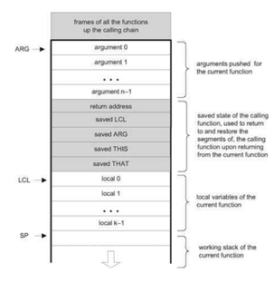
Figure 105 shows how a simple C function might be translated into VM code.

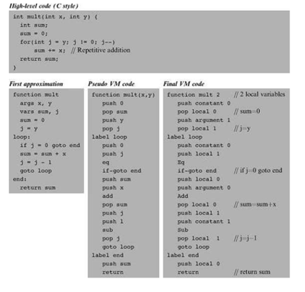
Compiler

The compiler used in this project translates code from the high-level programming language Jack into a VM code. The compiler was written in the Rust programming language and a link to the source code can be found in Appendix A.

Jack is a simple, weakly-typed, object-oriented language with most of the features present in popular modern programming languages. A Jack program consists of one or more classes. Each class must reside in its own .jack source file. The entry point for every Jack program is a function named main within a class named Main (case sensitive). A Jack class consists of a number of field and/or static variables and a number of subroutines. Each subroutine can be either a constructor, function or method. Jack has three primitive data types: integer, char, boolean. Alternatively, a variable may be of object class in which case it is actually a reference to an object on the heap. This means that programmers can define their own types using classes. There are four kinds of variables (which correspond with the VM memory segments): field, static, local and parameter each of which has an associated scope. Field and static variables must be declared at the start of a class usings the field and static keywords respectively. Local variables must be declared at the start of subroutines using the keyword var. Parameter variables are declared as part of a function declaration.

 Jack features five statements: let, if, while, do and return. If, while and return correspond to standard C-style statements. Let is used to set a variable to a value and do is used to call a subroutine and discard its return value. Jack also has recursively-defined expressions, however it does not define an operator precedent and therefore liberal use of brackets is encouraged.

Jack is a context-free grammar and only requires lookahead when determining whether a variable is a standard variable or an array. Conveniently, the VM layer already provides most of the memory management and function calling capabilities needed by the high-level language. Jack does not support overriding or inheritance which simplifies the compiler and means that tasks such as determining which methods belong to each instance of an object can be done statically.

Figure 106 - Figure 108 below show a number of example Jack programs.

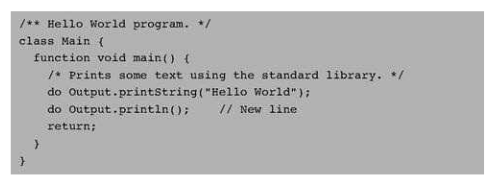
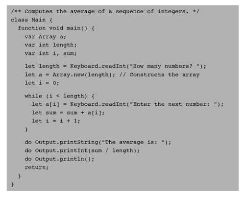
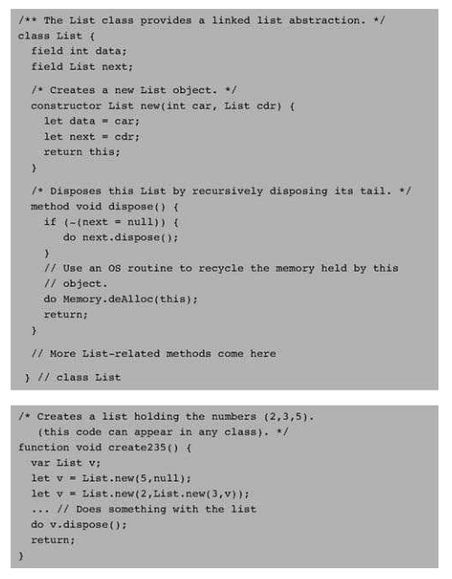
Operating System (OS)

The Operating System (OS) of a computer acts as a bridge between the hardware and software of a computer. It does this by interacting with the hardware of the computer and providing a number of services to programs running on the system. As the Hack platform is single-tasking and single-program it does not require a particularly complex OS and in fact the Hack OS may be closer to a standard library than an OS. With that said, it does provide a number of essential services which are divided into 8 categories (classes) and listed below:

·         Math: provides basic mathematical operations (multiply, divide, min, max, abs, sqrt)

·         String: implements String type and provides string-related operations (new, length, charAt, setCharAt, appendCHar, eraseLastChar, intValue, setInt, backSpace, doubleQuote, newLine, dispose)

·         Array: implements Array type and provides array-related operations (new, dispose)

·         Output: handles outputting text to the screen (moveCursor, printChar, printString, printInt, println, backSpace)

·         Screen: handles graphical output to the screen (clearScreen, setColor, drawPixel, drawLine, drawRectangle, drawCircle)

·         Keyboard: handles user input from the keyboard (keyPressed, readChar, readLine, readInt)

·         Memory: handles memory operations (peek, poke, alloc, deAlloc)

·         Sys: provides execution-related services (halt, error, wait)

Each of these classes are compiled into VM files and then the 8 VM files are included with each program.

Toolchain

Thus, the complete process from high-level Jack program to a Hack machine code binary that can be run on the system is summarised below:

1.       Compile the Jack program into VM code, one VM file per Class.

2.       Translate the VM files (including the 8 OS files) to a single assembly file

3.       Assemble the assembly file into a single binary

4.       Burn the binary to a ROM cartridge (or load into a simulator)

Appendix D: Software optimisations

The first challenge faced during this project was the size of the binaries produced by building Jack programs. Due to the 15-bit width of the ROM address bus, the maximum program size for the original Hack architecture is 32768 instructions. Although a 32-bit mode was added to the simulator to make it possible to run larger programs, initially attempts were made to reduce the size of the programs by optimising at the VM level. These attempts succeeded in reducing the size of smaller programs such as “Seven” to a size where they could fit into the original 32K ROM, however larger programs such as “Pong” still require the use of the 32-bit mode.

Naturally, each successive layer in the build process adds a level of overhead that increases the size of the produced binaries. Whilst there are surely further optimisations that could be made at the VM level that would further reduce the size of the binaries, there are also a number of other approaches worthy of consideration.

One approach that may substantially reduce the size of binaries produced by the build process is to remove the VM layer entirely and instead compile directly to assembly at the compiler level. This would necessitate the creation of a much larger and more complex compiler that would need to handle operations such as memory management itself, but would eliminate much of the overhead associated with the VM layer and produce tighter binaries. This would also eliminate all of the benefits associated with a VM layer such as the ease of porting other language compilers to the Hack platform.

The bulk of the code in a binary produced during the build process consists of OS code. Therefore, improving the efficiency of the OS code would help in reducing the size of the programs. One possible approach to this could be to manually rewrite the operating system in optimised assembly.

Replace Halt

Jack programs are terminated by calling an operating system procedure called Halt. Halt simply enters the system into an endless loop. However, as the Operating System was developed in Jack, an endless loop compiles down into a large number of assembly instructions, including checking that condition associated with the while loop still holds. This can be replaced by 3 assembly instructions. Compared to other optimisations, this does not make much of a difference to the program size, however, it does make it much easier for the simulator to detect the end of a program which is useful for measuring performance.

Dead Code Elimination

Dead Code Elimination (DCE) is a classic compiler optimisation technique in which functions that are never called are detected and removed from the program. Since the OS includes the entire standard library for the Jack program language, it is very rare for every included function to be called. Therefore, the removal of this dead code can significantly reduce the size of programs, especially when only a few of the OS functions are utilised. This optimisation builds an index of where functions start and end as well as if they are called or not. Once the index is complete, the functions that are not called are removed from the program. This optimisation is called repeatedly until no further functions are removed.

Increments

When a Jack program increments or decrements a variable by 1, a large number of instructions are produced, including pushing 1 onto the stack and then loading it into the D register. The Hack platform includes instructions to directly increment or decrement a register by 1. This optimisation uses a regular expression to search the program for the assembly produced by incrementing by one and then replaces these instructions with a tighter implementation that takes advantage of the increment/decrement assembly instructions.

Two Stage Increment

This optimisation looks for increments that occur across two instructions, when they can be combined into one. For example:

D=M
D=D+1

Can be optimised to:

D=M+1

Loading 0 or 1 into A

The Hack platform is able to use the ALU to set the value of a register directly to 0 or 1. However, programs produced by the VM translator layer will often load 0 or 1 into the A register and then perform arithmetic using the A register. For example:

@1
D=D+A

Can be optimised to:

D=D+1

Redundant A instructions

This optimisation looks for cases where a value that has already been loaded into the A register, is redundantly loaded again. This can be detected by looking for cases where an A instruction is repeated, with no code in between the first and second instances of the A instruction that changes the value of the A register. The repeated A instruction can simply be deleted.

Results

Figure 109 shows the number of static instructions when translated without any VM-level optimisations compared with using all 5 VM translator optimisations on each of the benchmarks. This graph shows a clear reduction in the number of instructions for every benchmark. Figure 110 shows the average effect of each of the 5 optimisations individually across all the benchmarks. Dead code elimination removes the most code and would have the biggest effect on programs that do not use many operating system functions. Both these graphs show that the VM-level optimisations have a substantial effect on executable size, around 25%