Branch Prediction Simulation

Abstract
This document discusses the results of a branch prediction simulation experiment. The simulator was implemented in C++ and supports 6 different prediction strategies. The results gathered are analyzed and discussed in order to assess the effectiveness of each strategy.
Introduction
Most modern CPUs utilise the so-called “5-stage pipeline” – splitting each instruction into 5 stages: Instruction Fetch (IF), Instruction Decode (ID), Execution (EX), Memory Access (MEM), Register Write Back (WB) [1]. The use of this pipeline enables Instruction Level Parallelism (ILP) by performing each of these stages simultaneously on different instructions; i.e. whilst Instructioni is in the WB-stage, Instructioni-1 is in the MEM-stage, Instructioni-2 is in the EX-stage and so on. This can offer dramatic performance improvements.
Branch instructions (which can be thought of as low-level if statements) introduce a challenge for the 5-stage pipeline. When a branch instruction is encountered, the CPU must either set the Program Counter (PC) to the target of the branch instruction if the branch is taken, or must increment the PC to the next value if the branch is not taken. However, the CPU does not know if the branch has been taken or not until the EX-stage, which leads to the potential that the IF-stage fetches the wrong instruction. The simplest way to deal with this is to stall the pipeline until the outcome of the branch is known, but this wastes valuable cycles.
Although many solutions to this problem have been proposed, this document concerns itself with the “branch prediction” method. Under this method, the CPU attempts to guess the outcome of the branch – taken or not taken. It then continues to process the pipeline under the assumption that it’s guess was correct, i.e. it fetches the instruction at the branch target if it predicted taken or it fetches the instruction at PC+1 if it predicts not taken. Once the outcome of the branch is known, if the prediction was correct, execution continues as normal. If the prediction was wrong, the CPU incurs a penalty as it has to stop execution and go back to fetch the correct instruction. The performance of such an approach is heavily dependent on the prediction strategy used.
This document discusses 7 predictions strategies: Always Taken, 2-bit (Bimodal), Global History with Index Sharing (Gshare) and 3 different profile-based strategies. These strategies, as well as their implementation details in the simulator, will be discussed later in this document.
The remainder of this document contains a brief discussion on the simulator, an outline of the prediction strategies as well as any relevant implementation details, details on the methodology of the experiments, a presentation of the results, an evaluation of the prediction strategies and finally a conclusion answering the research questions posed in the methodology section. The appendix of this document contains the raw results from the experiments.
Simulator
The simulator on which the experiments in this document were preformed is a C++ program. The program operates on branch trace files which are text documents where each line contains two values separated by a space. The first value is a branch address, and the second value is bit indicating if the branch was taken or not taken. These trace files are considered the ground truth during the simulation, and the predictions of the various strategies are compared against this ground truth. The author had access to 30 branch traces. A python script was also developed to run the simulator using multiple strategies across multiple trace files as a batch and generate a CSV of results.
The simulator follows this procedure:
- Collect trace file path and prediction strategy (as well as any other options) from the user in the form of command line arguments and display an error and usage message if these are not provided correctly.
- Load the trace file into a BranchTrace data structure that allows accessing the branch address and branch outcome as well as comparison between BranchTraces. This initial BranchTrace will be referred to as the “ground truth”.
- Instantiate a predictor object of the selected prediction strategy.
- Feed the branch addresses from the ground truth one by one into the predictor object. Once the predictor object has made a prediction it is recorded in a second BranchTrace object and the predictor is then told the actual outcome of the branch.
- Once all instructions have been passed into the predictor, the prediction BranchTrace is compared against the ground truth BranchTrace and the results are printed to the console.
- Any options (such as print to file) are carried out.
The complete source code for the simulator, as well as the trace files used can be viewed here: https://git.jbm.fyi/jbm/Branch_Prediction_Simulator.
Prediction Strategies
Always Taken
Always taken is the simplest of the prediction strategies. Under this strategy, the CPU will always predict that a branch is taken, without taking into account any dynamic information. This will mean that on average, the prediction will be correct around half the time, although this statistic can be improved if the compiler is aware of this strategy and optimises the code to take advantage of it.
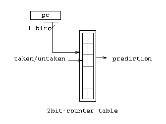
2-bit (Bimodal)
The 2-bit strategy responds dynamically to the outcomes of previous branches. Under this strategy, the CPU maintains a prediction table of size n.The table is indexed by the last log2(n) bits of the branch instruction address, e.g. if the table has 512 entries, then the last 9-bits of the branch address will be used to index the table. Each entry is a 2-bit counter. Every time a branch address is taken, its respective counter will be incremented and every time it is not taken, the counter will be decremented. The predictor then uses the upper bit of the relevant counter to make its prediction:
Decimal = 0, Binary = 00, Predict: not taken
Decimal = 1, Binary = 01, Predict: not taken
Decimal = 2, Binary = 10, Predict: taken
Decimal = 3, Binary = 11, Predict: taken
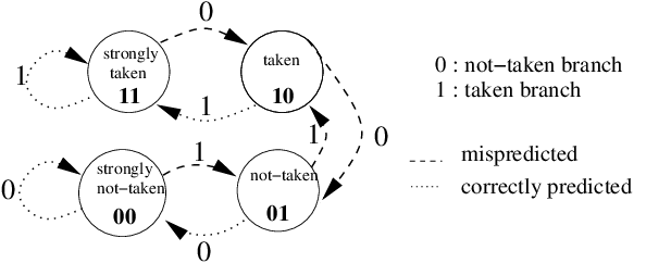
The upper bit of the counter is known as the prediction bit, and the lower bit as the conviction or hysteresis bit. This 2-bit scheme means that the predictor needs to be wrong twice in a row in order to change its prediction, which helps to stabilise the strategy when compared to a 1-bit counter.
As only a subset of the address is used to index the table, there will be multiple address that map to the same entry in the table. In the simulator, this prediction table has been implemented as an array of chars. Every time a value v in the table is updated, it is constrained such that v >= 0 and v <= 3.
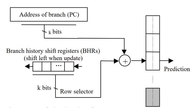
GShare
The GShare strategy is similar to the 2-bit strategy but also takes into account that previous branches may affect the outcome of future branches, even if those branches do not share an address. Gshare maintains the same n-sized prediction table with 2-bit counters as the 2-bit strategy, but also maintains a global history register (GHR). This register is shifted left each time a branch occurs, and the last bit of the GHR is set to 1 if the branch was taken and 0 if it was not. The strategy then proceeds in the same way as the 2-bit strategy, only the table is indexed by the last n-bits of the branch address XOR the last m-bits of the GHR. Note that n and m do not need to be equal, but in these experiments they will be.
In the simulator, the prediction table is implemented the same as in the 2-bit strategy. The GHR is implemented as a class with a history()and update(bool taken) method. The class contains an unsigned long representing the register. The history method simply returns this long, whilst the update function uses bitwise operations to shift the register to the left and set the final bit to the value of the taken Boolean variable.
Profile-based approaches
Profile-based approaches allow the predictor to view the code in a “profile” run before the “real” run. The predictor must come up with some way of representing the insights of the profile run which can be utilised in the real run. Three different profile strategies were experimented with.
Section Profile
In the “section profile” strategy, the predictor maintains an n-entry Boolean prediction table. During the profile run, the branch trace is split into n equal (or nearly equal if the total instructions are not divisible by n) sections. For each section a “mini-profile” is generated which records the total number of branch instructions, the number of taken branches and the number of not taken branches. Each mini-profile is mapped to an entry in the prediction table which is set to 0 if there were more not taken branches then taken branches, and 1 if there were more taken branches.
During the real run, the prediction strategy then acts similarly to the always taken strategy, only it changes between always taken and always not taken based on which outcome is more likely for the current section. The outcome to use is determined by using the instruction index / (total instructions / n) as an index for the prediction table.
In the simulator, this was implemented using a dedicated Profiler class which traverses the ground truth table and generates n mini-profiles. These mini-profiles are then passed to the SectionProfile class which populates a Boolean prediction table with the values determined by comparing the taken to not taken values from each profile. Due to poor performance, and the reasons discussed in the next paragraph, this strategy was removed from the simulator, however the code remains in the repository.
This strategy is unlikely to be easy to implement in real hardware, as it requires the predictor to be aware of the instruction index of the current instruction within the program, instead of the branch address as the other predictors use.
Predetermined
In the “predetermined” strategy, the predictor maintains also an n-entry Boolean prediction table. The prediction table is addressed in the same way as in the 2-bit strategy, using the last log2(n) bits of the branch address as the index for the prediction table.
However, unlike in the 2-bit strategy, the table is prepopulated with either 0 or 1, based on which outcome is more plentiful for each address, during the profile run of the code. During the real run of the code, the relevant prediction is retrieved from the prediction table and no updates occur during the runtime. The lack of an update step means that in theory, there will be less runtime overhead. However, this fact is of course counter-balanced by the need to run a profile of the code prior to real execution of the code.
In the simulator, this strategy is implemented by creating an integer table of counters, using the same addressing scheme as the Boolean table discussed above. The ground truth is then iterated through incrementing the relevant counter for each branch that has a taken outcome, and decrementing for each branch that is not taken. Once this is done, the integer table is transferred over to the Boolean table by setting the relevant address to 0 if the corresponding integer value is negative and 1 if the corresponding integer value is positive.
If implemented in real hardware, the same method as described above could be used, storing the integer values either in the CPU cache or in main memory. If the performance of the profile run is not relevant, there is no need for dedicated hardware to perform profile step of the strategy. A strategy similar to this could be useful if the runtime performance of the code is vital, but there is time to prepare a profile prior to the real run.
Predetermined Global
The “Predetermined Global” strategy is very similar to the Predetermined strategy, only it also makes use of the GHR as in the Gshare strategy. This means that the strategy incorporates some dynamic information as well as making use of the predetermined static values.
The profile run of the code is performed in the same way as the Predetermined strategy, but also tracks the state of the GHR during the profile. The prediction table is indexed using the last n-bits of the branch address XOR the last m-bits of the GHR. The real run of the strategy is also performed in the same way as the Predetermined strategy, but the predictor must also update the GHR in real time, which reintroduces some of the overhead done away with in the Predetermined strategy.
The implementation in the simulator and in real hardware would be done in the same way as described for the Predetermined strategy but also incorporating the GHR.
Methodology
Performance statistics for each of the strategies across each of the 30 trace files were gathered by running the simulation across each combination of prediction strategy and trace file. This process was automated using a python script, resulting in a single CSV of data. This raw data can be seen in the appendix of this document.
With this data gathered two research questions were formulated:
Question 1: Which prediction strategies yield the best performance?
Question 2: What is the effect of table size on performance?
These questions were answered using statistical analysis of the results and these results are presented in a number of graphs, shown in the results section below.
Results
On the following charts, the strategy names have been abbreviated. See the table below for a description of what each of the abbreviations stand for, as well as the mean, median and range of each of the strategies (these will be plotted later).
Strategy |
Description |
MEAN |
MEDIAN |
RANGE |
A |
Always Taken |
55.93027667 |
52.30975 |
38.4204 |
S512 |
2-Bit with table size 512 |
90.57706667 |
89.42695 |
20.925 |
S1024 |
2-Bit with table size 1024 |
91.54628 |
91.31485 |
20.925 |
S2048 |
2-Bit with table size 2048 |
92.11433333 |
92.05795 |
20.925 |
S4096 |
2-Bit with table size 4096 |
92.35294 |
92.60495 |
20.925 |
G512 |
Gshare with table size 512 |
89.48314 |
87.81435 |
16.1721 |
G1024 |
Gshare with table size 1024 |
90.81912667 |
88.5667 |
14.0014 |
G2048 |
Gshare with table size 2048 |
91.82763667 |
90.29995 |
12.983 |
G4096 |
Gshare with table size 4096 |
92.37427 |
91.5656 |
12.8358 |
P512 |
Predetermined with table size 512 |
88.97668667 |
88.90865 |
23.5955 |
P1024 |
Predetermined with table size 1024 |
90.93857333 |
90.8176 |
19.0689 |
P2048 |
Predetermined with table size 2048 |
92.28933333 |
92.3603 |
18.1857 |
P4096 |
Predetermined with table size 4096 |
93.08119 |
93.08655 |
18.0499 |
PG512 |
Predetermined Global with table size 512 |
86.02312333 |
84.9818 |
30.7332 |
PG1024 |
Predetermined Global with table size 1024 |
88.73319333 |
88.1564 |
27.0943 |
PG2048 |
Predetermined Global with table size 2048 |
91.04037667 |
91.5198 |
22.8168 |
PG4096 |
Predetermined Global with table size 4096 |
92.69009667 |
93.04445 |
18.9531 |
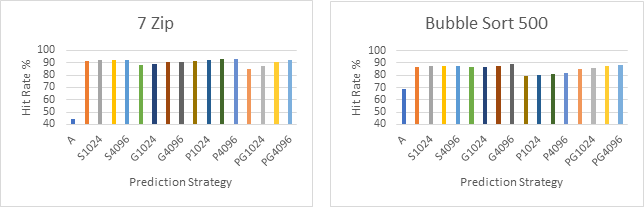
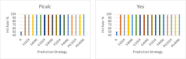
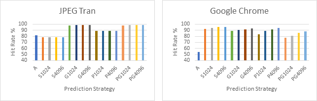
Six of the sample branch traces (7Zip, Bubble Sort 500, Picalc, Yes, JPEG Tran and Google Chrome) were selected to compare the performance of each strategy on that trace:
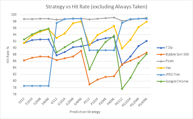
Next all six of these traces are plotted on the same line graph with the A strategy excluded to offer a higher resolution look at the performance differences between the more complex strategies.
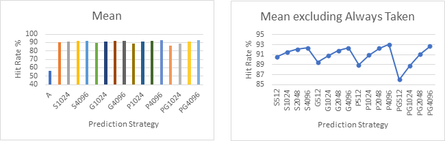
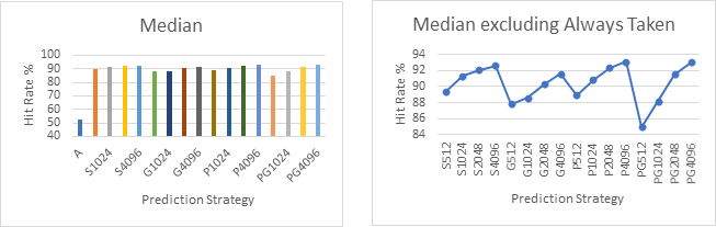
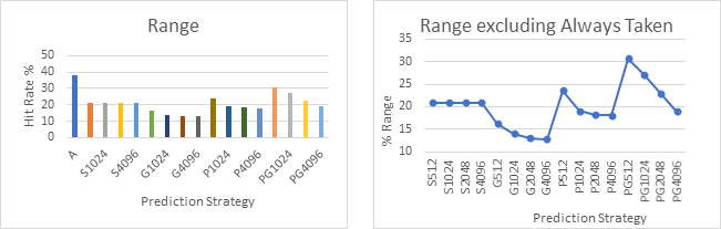
The next graphs show the mean, median and range of each of the strategies across all 30 sample branch traces plotted as bar charts and line graphs. The line graphs on the right exclude the A strategy to offer a higher resolution look at the more complex strategies.
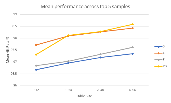
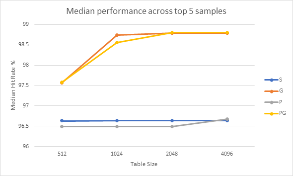
Next, the mean and median performance of the more complex strategies is shown across the top five performing samples for the respective strategy. This allows us to see the performance of the strategies in their best (or near best) case scenarios, and allows a tertiary look at performance across table size.
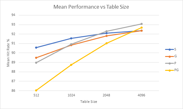
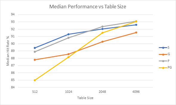
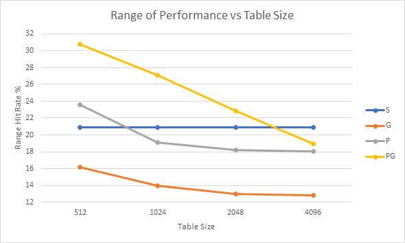
Finally, the impact of table size of on performance is directly analysed. The charts below show the performance in terms of mean hit rate, median hit rate and hit rate range for each of the strategies across all of the samples vs table size.
Evaluation
By looking at the first six graphs, which compare the performance of the different strategies on the same branch trace, we can see that the Always Taken strategy consistently performs much worse than the dynamic strategies. This is not surprising as dynamic strategies generally perform better then static strategies as they make use of more up to date information. However, it should be noted that the compiler is unlikely to have optimised for the Always Taken strategy in this case and therefore it is likely that better performance could have been achieved had the compiler been aware that this strategy was in use.
Graph 7 shows the same data at the first 6 graphs but on the same chart and excluding the Always Taken strategy. This gives us a higher resolution look as the dynamic strategies. This chart shows that the performance of all the strategies is highly correlated with the sample itself, i.e. if one strategy performs well it is likely that all strategies will perform well. This is clearest on the Picalc series, but one can note that all the other series follow roughly the same pattern. This suggests that the biggest impact on performance is not the prediction strategy used, but the predictability of the branches within a sample. This may lead to average metrics, such as median and mean being misleading when applied across the whole sample set.
Graphs 8 – 11 shows the average performance of each strategy across the entire sample set. Charts 9 and 11 clearly show that performance improves as the table size increases, which is again unsurprising as these strategies have access to more information. The best overall performance across all the samples seems to be achieved by the Predetermined Strategy with a table size of 4096. However, it has only narrowly beaten the standard 2-bit strategy and the Gshare strategy with the same table sizes, neither of which require a profile run of the code.
When looking at graphs 12 and 13, which shows the range in performance achieved by the various strategies, lower values indicate a more consistent performance. Here, Gshare is the clear winner with none of the other strategies able to offer more or even close to the consistency of Gshare.
Graphs 14 and 15 show the mean and median performances respectively of the various dynamic strategies across the top 5 samples for each respective strategy. This allows us to observe the strategies in their best-case scenarios across the sample set. Here we can see that the Standard 2-bit strategy and the Predetermined strategy offer similar performance to each other, whilst the Gshare and Predetermined Global strategies offer similar performance to each other. This is not surprising as these pairs of strategies are similar to each other. Generally, the Predetermined strategies offer slightly higher performance, however this is counter-balanced by their need to perform a profile run of the code before the real execution can begin. Gshare is able to show a performance advantage against Predetermined Global when the table size is 512 and when looking median graph, the Standard 2-bit prediction beats the Predetermined strategy for all table sizes lower than 4096. These facts further show that the Predetermined strategies are unlikely to be worthwhile.
Graphs 16 – 18 show a clear trend of improved performance and consistency as table sizes increase. At lower table sizes it seems that the standard 2-bit strategy has the best performance whilst at larger table sizes the Predetermined strategies begin to show better performance. At higher table sizes Gshare and the Standard 2-bit strategies offer similar performance to each other, but Gshare is substantially more consistent.
Conclusion
The results gathered in this project are able to offer a clear answer to question 2: increased table sizes offer increased performance. It would be interesting to repeat the experiments for more table sizes to see if the performance continues to increase with table size, or if it begins to plateau.
The answer to question 1 is less clear cut. The Gshare strategy is able to offer better performance than the Standard 2-bit strategy when only looking at the strategies in their best-case scenarios, but seem to offer similar performances across the entire sample set. Gshare is also is also able to offer a more consistent performance, so it’s probably fair to say that Gshare outperforms the Standard 2-bit strategy and does so without incurring significantly higher overhead. It would be interesting to repeat this experiment across more samples to see if these trends hold out.
The Predetermined Global strategy was able to offer similar or better performance to the Gshare strategy, but only at larger table sizes. As the Predetermined Global strategy requires a profile run of the code before any “real” execution can begin, this overhead is unlikely to be worthwhile for many applications. However, if there is time to prepare a profile but real execution must be highly optimised, it may make sense to use this strategy in some settings.
References
[1] J. L. Hennessy, David A. Patterson 2012: “Computer Architecture: A Quantitative Approach”, 5th Edition, Appendix C.
[2] C. Maiza, C. Rochange, 2006: “History-based Schemes and Implicit Path Enumeration”.
[3] Z. Su, M. Zhou, 1995: “A Comparative Analysis of Branch Prediction Schemes”.
[4] N. Ismail, 2002: “Performance study of dynamic branch prediction schemes for modern ILP processors”.
Links
PDF Version: https://www.jbm.fyi/static/branchprediction.pdf
Code/Traces: https://git.jbm.fyi/jbm/Branch_Prediction_Simulator